How to use this manual
This manual explains every page of GeoCAD Bridge (https://www.geocadbridge.com) and how to work with it. Each chapter covers one page or one family of pages: what it is for, how to use it step by step, a worked example, and links to the templates you need.
The Workspace is described last, in Part 3, because it is the largest tool on the site and needs a full explanation of every tab, command and panel.
| Part | Contents |
|---|---|
| Part 1 · Getting started | The site, the navigation bar, the home page and the tools hub |
| Part 2 · Site pages | Coordinate tools, EPSG and CRS reference, survey tools, field tools, file converters, Knowledge Center, resources and templates, help pages, Arabic pages |
| Part 3 · Workspace | Layout, projects, coordinate systems, import and export, every ribbon tab and command, the command line, survey panels, worked examples |
| Appendices | Template downloads, keyboard shortcuts, troubleshooting |
Conventions used in this manual
- Button and field names are written in bold exactly as they appear on screen, for example Run Adjustment.
- A path such as Survey › Surfaces › Point Groups means: open the Survey ribbon tab, find the Surfaces group, click Point Groups.
- Web addresses are given relative to the site, for example
/traverse/means https://www.geocadbridge.com/traverse/. - Coordinates are written Easting, Northing (E, N) for projected systems and longitude, latitude for geographic systems unless stated otherwise.
Part 1 · Getting started
About GeoCAD Bridge
GeoCAD Bridge is a browser-based platform for surveyors, GIS analysts and CAD engineers. It takes data from Civil 3D, Trimble Business Center, ArcGIS Pro, QGIS, total stations and GNSS receivers, processes and corrects it, and exports it to any other program in the right coordinate system.
Your files stay on your device. Every calculation runs inside your browser. Files you open are read locally and are not uploaded to be processed. Projects are kept in your browser’s storage until you export them. The only things that leave your device are what you send on purpose (for example a support e-mail) and standard usage analytics.
What you need
- A current browser: Google Chrome or Microsoft Edge (desktop or Android) are tested. Firefox and Safari use the same web standards.
- An internet connection for the first visit and for basemap tiles. After the first visit the main tools can keep working with a weak connection.
Installing it as an app. The site can be installed like an app and then opens without the browser toolbar:
- Chrome / Edge on a computer: click the install icon at the right of the address bar, or the browser menu › Install GeoCAD Bridge.
- Android: browser menu › Add to Home screen.
- iPhone / iPad (Safari): Share › Add to Home Screen.
Accuracy statement. Projection mathematics follow the EPSG Dataset via PROJ 9.5.1. Datum changes use the published Helmert (towgs84) parameters of each coordinate reference system (CRS), so their accuracy is that of those parameters (from decimetres to several metres; it is shown for each CRS in the EPSG Library and CRS Toolkit). Grid-shift files (NTv2, NADCON, geoid models) are not applied, and heights are passed through unchanged unless a tool says otherwise. For legal or cadastral work, confirm parameters with your national mapping agency and check one known control point.
The navigation bar
Every content page has the same navigation bar at the top.
| Item | What it opens |
|---|---|
| GeoCAD Bridge logo (rotating globe) | The home page / |
| Home | The home page |
| Survey Tools ▾ | All Tools Hub /tools/, Traverse Adjustment /traverse/, Survey Calculators /survey-calculators/, Coordinate Transformation /coordinate-transformation/ |
| Coordinate Systems ▾ | Coordinate Systems hub /coordinate-systems/, EPSG Library /epsg/, EPSG Finder /coordinate-transformation/?mode=epsg, country pages for Saudi Arabia, Egypt, UAE and Qatar |
| Field Survey | Field Visit Survey /field-visit-survey/ (a direct link: it is the one field page) |
| CAD/GIS Converters ▾ | SHP to DXF /shp-to-dxf/, SHP to KMZ /shp-to-kmz/, KMZ to DXF /kmz-to-dxf/, DXF to KMZ /export-dxf-to-kmz/, GeoJSON to KMZ /geojson-to-kmz/, CSV Points to KMZ /csv-point-to-kmz/, Batch Coordinate Converter /coordinate-transformation/?mode=batch, Workspace Converters /workspace/ |
| Resources | Resources & Templates /resources/ |
| Help ▾ | Help Center /help/ with the How to Use guides (Workspace, Traverse Adjustment, Coordinate Transformation, Field Survey, File Converters, EPSG Reference), the User Guide /help/user-guide/ (this manual as a web page, in English or Arabic), Support, About, Keyboard Shortcuts, What’s New, and the Knowledge Center /knowledge/ |
| Search icon 🔍 | Opens the All Tools Hub, where tools can be filtered |
| Sign In | Opens the account login window. The login service is not activated yet: the window is a preview only and does not send or store a user name or password |
| Open Workspace | The GIS/CAD Workspace /workspace/ (Part 3) |
Pages that have an Arabic version show an العربية link that switches to the same page under /ar/ (see chapter Arabic pages). Full-screen application pages (Traverse, Coordinate Transformation, Field Visit Survey, the six file converters and the Workspace) replace this bar with their own compact header that still links back to the home page through the logo.
Home page /
The home page is the starting point for the four main tools and the six one-page file converters.
What is on the page
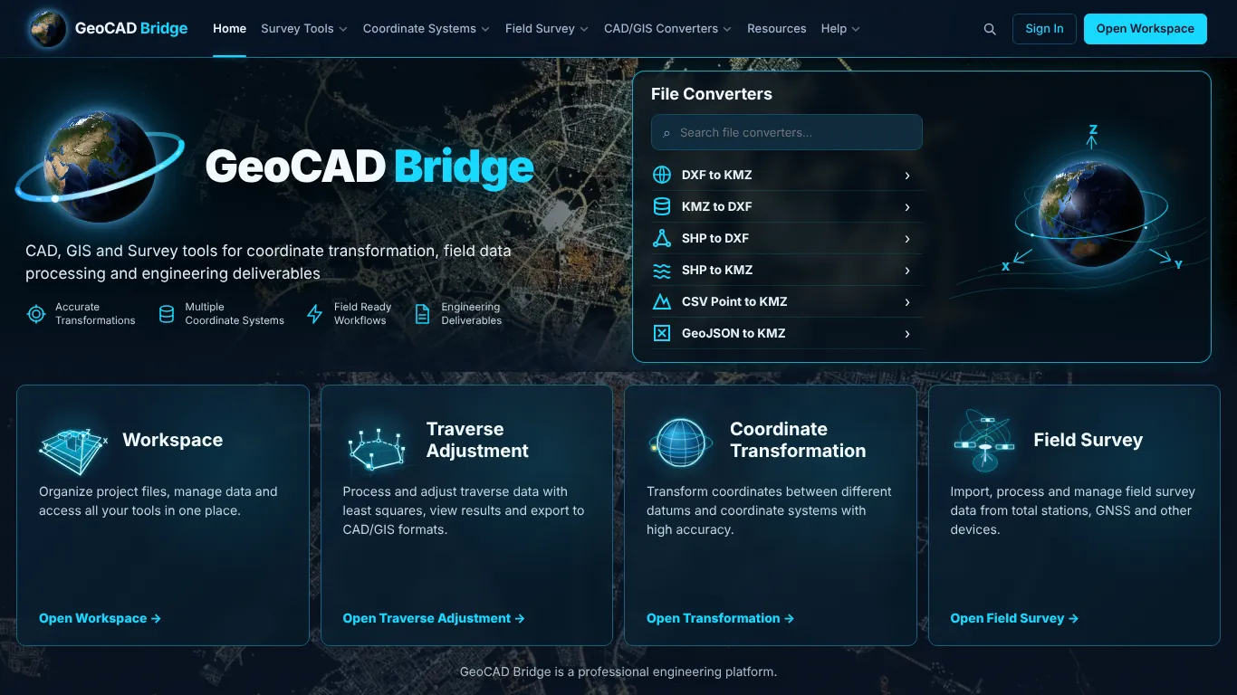
- Hero: the GeoCAD Bridge title with the rotating globe and four promises: Accurate Transformations, Multiple Coordinate Systems, Field Ready Workflows and Engineering Deliverables.
- File Converters panel (right): a search box Search file converters… and direct links to DXF to KMZ, KMZ to DXF, SHP to DXF, SHP to KMZ, CSV Point to KMZ and GeoJSON to KMZ. Type part of a name to filter the list.
- Four tool cards with an Open … link each:
- Workspace – organise project files, manage data and reach all tools in one place →
/workspace/. - Traverse Adjustment – process and adjust traverse data, view results and export →
/traverse/. - Coordinate Transformation – transform coordinates between datums and systems →
/coordinate-transformation/. - Field Visit Survey – record site visits, points, photos and reports →
/field-visit-survey/.
- Workspace – organise project files, manage data and reach all tools in one place →
How to use it. Click the card of the job you want to do. If you only need to change a file from one format to another, use the File Converters panel. Adding #sign-in or #help to the home page address (/#help) opens the login window or the quick Help window directly.
The quick Help window on the home page lists the recommended order of work, which applies to every tool on the site:
- Choose the module from the navigation bar.
- Select the project CRS before importing or processing data.
- Use the correct template for points, traverse observations or batch coordinates.
- Validate the data before exporting deliverables.
All Tools Hub /tools/
The Survey Tools Hub lists every tool as a card with its category, status and an Open Tool → button.
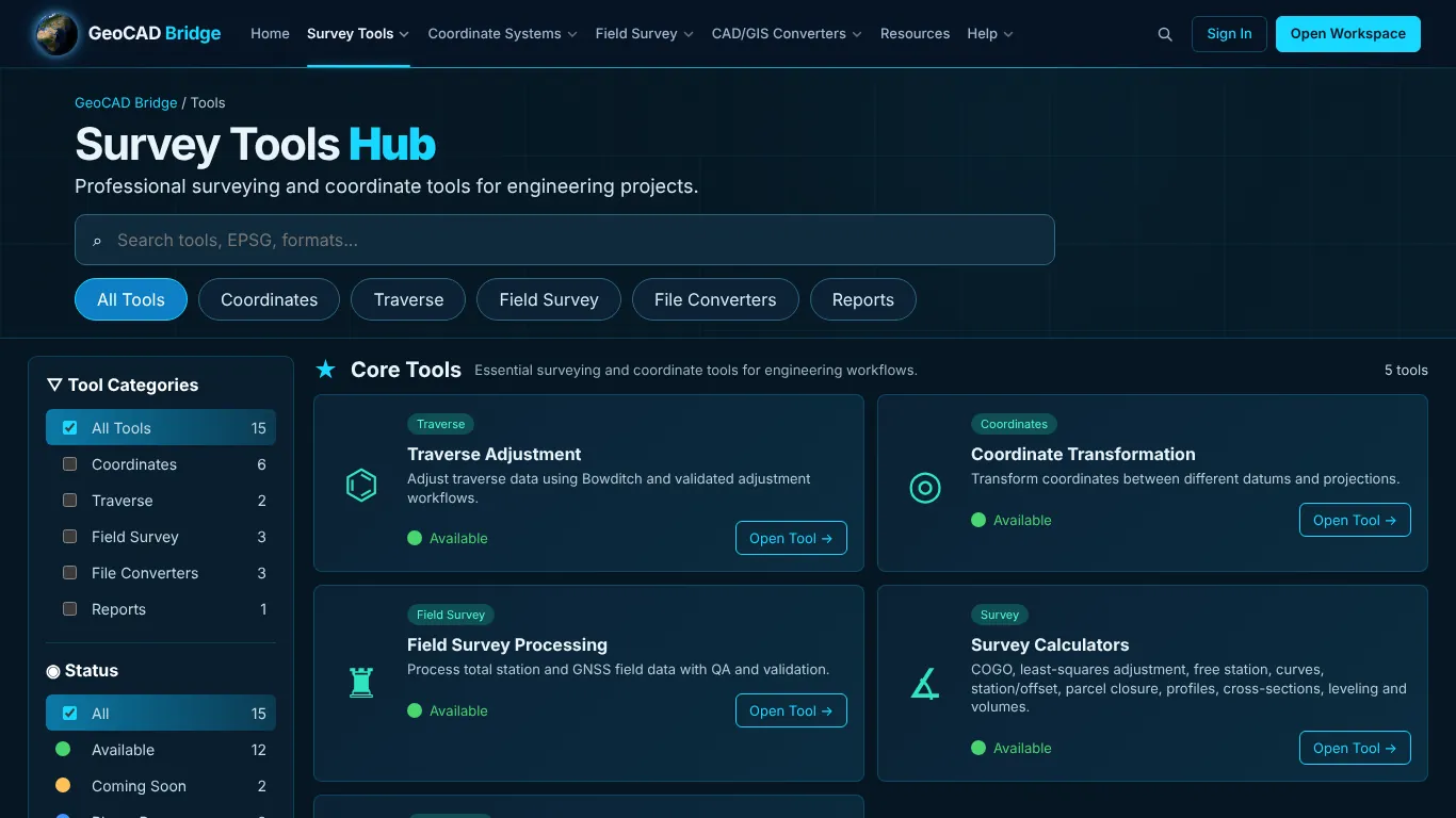
Filters (left column)
- Tool Categories: All Tools, Coordinates, Traverse, Field Survey, File Converters, Reports.
- Status: All, Available, Coming Soon, Phase B.
- Data Type: Points / Coordinates, Traverse / Control, Field Data, Vector Files, Reports / Documentation.
Sections and cards
| Section | Card | Opens |
|---|---|---|
| Core Tools | Traverse Adjustment | /traverse/ |
| Coordinate Transformation | /coordinate-transformation/ |
|
| Field Visit Survey | /field-visit-survey/ |
|
| Survey Calculators | /survey-calculators/ |
|
| CRS Toolkit | /crs-tools/ |
|
| Field Data Tools | Field Visit Mapping | /field-visit-survey/ |
| Survey QA/QC (Phase B) | QA tools in the Workspace | |
| Field Site Mapping | Workspace | |
| Quick Converters | WGS84 to UTM | /coordinate-transformation/?mode=wgs84-to-utm |
| UTM to WGS84 | /coordinate-transformation/?mode=utm-to-wgs84 |
|
| EPSG Finder | /coordinate-transformation/?mode=epsg |
|
| Batch Coordinate Converter | /coordinate-transformation/?mode=batch |
|
| File Converters | CSV to KML, GeoJSON Viewer (DXF to KML is marked Coming Soon on this page; use /export-dxf-to-kmz/ instead) |
Workspace and converter pages |
The right column shows the Recommended Workflow (Import Data → Select CRS → Validate → Export) and Download Templates links:
- Field / point template (CSV): https://www.geocadbridge.com/downloads/Field_Visit_Points_Template.csv
- Traverse input template (Excel): https://www.geocadbridge.com/downloads/GeoCAD_Bridge_Traverse_Input_Template.xlsx
- All templates:
/resources/
Part 2 · Site pages
The coordinate library
Every page that asks for a coordinate system uses the same picker: the coordinate library (مكتبة الإحداثيات). In place of a long list, the page shows a button with the chosen system, for example UTM84-38N · UTM-WGS 1984 datum, Zone 38 North, Meter. Click it to open the library. This applies to the source and target systems of Coordinate Transformation, the quick converters, the country pages, the file converters, Field Visit Survey and the Workspace (new project, project CRS, layer CRS and Reproject Layer).
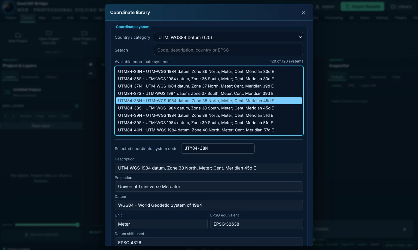
- Choose a Country / category on the left (for example Saudi Arabia, Egypt or UTM, WGS84 datum), or All coordinate systems (search).
- Type in Search: a code (
UTM84-38N), part of a description, a country or an EPSG number (32638). - Click a system in Available coordinate systems. The panel shows its Description, Projection, Datum, Unit, EPSG equivalent and the Datum shift used.
- Click OK. The button now shows the chosen system.
The library holds about 8,800 coordinate systems, of which about 8,350 can be converted. Systems marked Shown for reference use a projection or datum transformation the site cannot apply yet. On a country page or a country converter, the library opens on that country.
Coordinate Transformation /coordinate-transformation/
The main coordinate tool. It converts a single point or a whole table between any two of the 138 bundled CRS definitions (geographic WGS 84, NAD83, ETRS89, Web Mercator, all WGS 84 UTM zones north and south, KSA-GRF17, Ain el Abd 1970, MTRF-2000, Egypt 1907 belts and more), shows the point on a map, and explains which operations were applied.
Page layout
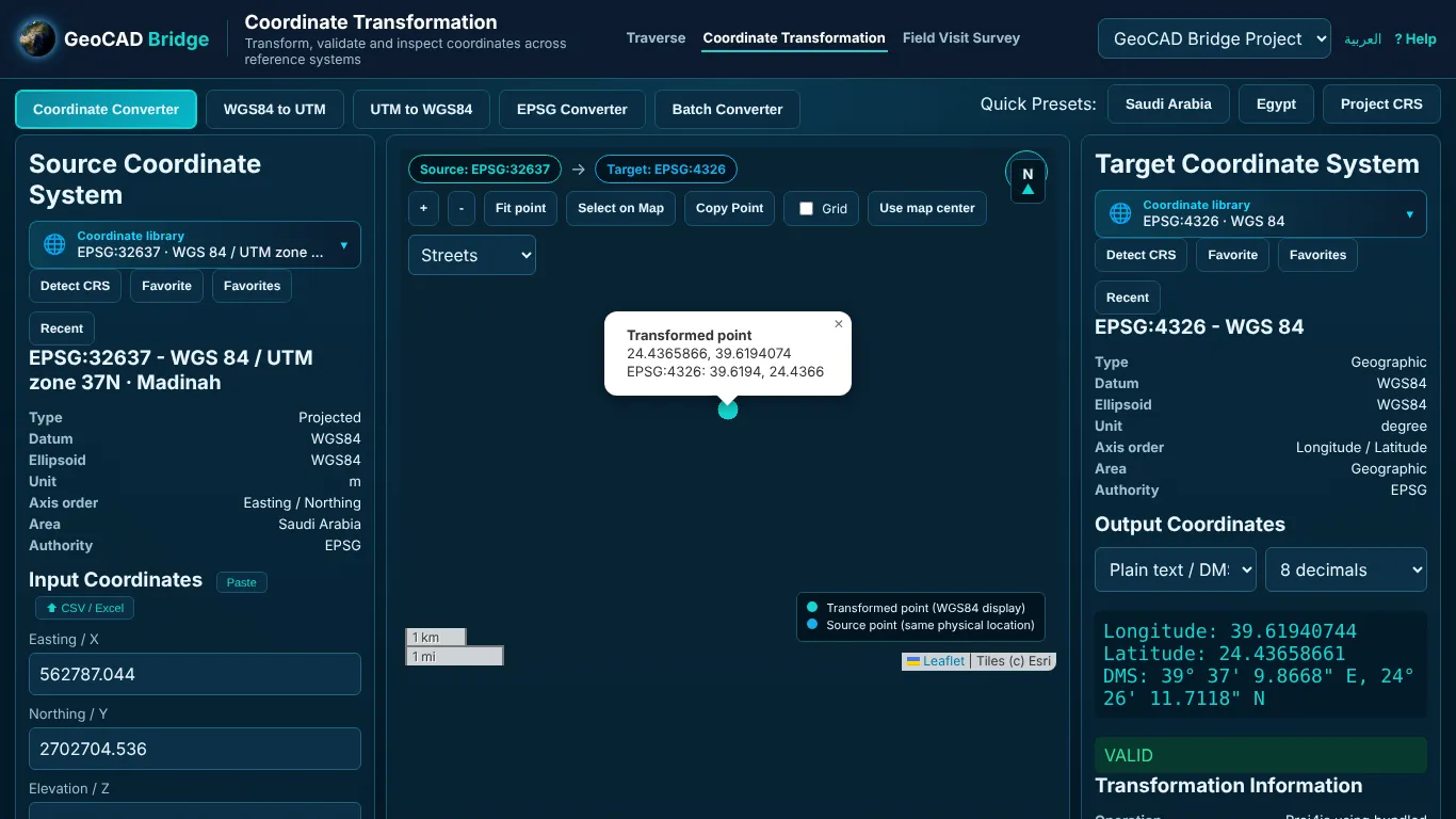
- Header: a compact bar with the GeoCAD Bridge globe, the page title, links to Traverse, Coordinate Transformation and Field Visit Survey, the active project, the language switch and Help.
- Mode buttons across the top: Coordinate Converter, WGS84 to UTM, UTM to WGS84, EPSG Converter, Batch Converter. The same modes can be opened with
?mode=wgs84-to-utm,?mode=utm-to-wgs84,?mode=epsg,?mode=batch. - Quick Presets: Saudi Arabia, Egypt and Project CRS set typical source/target pairs in one click.
- Active project selector (top): results can be kept with a named project.
- Source Coordinate System (left) and Target Coordinate System (right). Each has a Coordinate library button (see The coordinate library), Detect CRS, Favorite, Favorites and Recent. The selected system’s card shows Type, Datum, Ellipsoid, Unit, Axis order, Area and Authority.
- Input Coordinates: Easting / X, Northing / Y, Elevation / Z (or longitude / latitude for geographic systems), with Paste, ⬆ CSV / Excel (many points at once, see below), a Geographic format choice (Decimal Degrees or DMS / hemisphere notation) and the ⇄ button that swaps source and target.
- Map: shows the source and transformed point (same physical location) with + / −, Fit point, Select on Map, Copy Point, Use map center, a Grid overlay and a basemap list (Streets, Satellite, Hybrid, Terrain, Light, Dark, None).
- Output Coordinates with output format (Plain text / DMS, GeoJSON, WKT, CSV row) and precision (8, 6, 4 or 2 decimals).
- Transformation Information tabs: Results, CRS Details, Transformation Pipeline, Validation, History.
- Batch Conversion panel and action buttons: Preview & Transform, Download Results, Clear, Save Preset, Copy Results, Export CSV, Export Excel, ▶ Transform Coordinates.
How to convert one point
- Under Source Coordinate System, click the Coordinate library button, find the system (for example
UTM84-38N,32638orAin el Abd) and click OK. Use Detect CRS if you are not sure: it suggests systems that fit the numbers you typed. - Choose the Target Coordinate System the same way, from the same library. ⇄ swaps the two. Mark systems you use often with Favorite.
- Type the coordinates. For geographic input choose decimal degrees or DMS (for example
24° 30′ 00″ N). Y is latitude (north) and X is longitude (east). Z is optional and is kept unchanged unless a verified vertical operation exists. - Click ▶ Transform Coordinates (or press Enter). The result appears in Output Coordinates and on the map.
- Open Transformation Pipeline to see the steps used (inverse projection, datum shift, forward projection) and Validation for range and area-of-use checks.
- Copy Point / Copy Results put the result on the clipboard; Export CSV / Export Excel save it. Save Preset keeps the source/target pair for next time.
Worked example (WGS 84 to UTM zone 38N). Source EPSG:4326, target EPSG:32638. Enter longitude 46.5, latitude 24.0. Result: E = 652 578.355 m, N = 2 655 039.017 m. The point scale factor is 0.99988755 and the grid convergence +0.610223°. (These are the reference values published on the EPSG:32638 page of the site.) A direct link that pre-selects the pair is /coordinate-converter/?from=4326&to=32638. On this page, /coordinate-transformation/?source=EPSG:4326&target=EPSG:32638 does the same (library codes such as ADSK:UTM84-38N also work).
How to convert many points from a CSV file
- Choose the source and target systems as above.
- Click ⬆ CSV / Excel next to Paste and choose a CSV or Excel file with one point per row (Point ID, X / Easting / Longitude, Y / Northing / Latitude, optional Z). The template below has the right columns.
- The page switches to batch mode and converts every row at once. The results table shows each point with its status.
- Click the ⬇ CSV link under the results to download the converted file, or Excel for an .xlsx copy. The file has the columns point, sourceCRS, sourceX, sourceY, targetCRS, targetX, targetY, z, status and message.
How to convert a table (batch)
- Click Batch Converter (or open
/coordinate-transformation/?mode=batch). - Download a template: Excel template https://www.geocadbridge.com/downloads/Coordinate_Transformation_Batch_Template.xlsx or CSV template https://www.geocadbridge.com/downloads/Coordinate_Transformation_Batch_Template.csv. The columns are
Point ID, Easting / Longitude / X, Northing / Latitude / Y, Elevation / Z. - Drop the file on Drop or choose Excel/CSV or click to choose it.
- Check the column mapping: Point ID, X / Easting / Longitude, Y / Northing / Latitude, Z / Elevation.
- Select source and target systems, then Preview & Transform.
- Download Results (CSV or Excel).
Good to know. Datum shifts between old local datums and WGS 84 can be several metres; read Accuracy and datum limitations at the bottom of the page before survey-grade work. If a converted point appears in the sea, the axis order or the source CRS is usually wrong.
Quick coordinate converters
Nine single-purpose pages use the same converter engine with a simpler form. All have the same layout: From CRS and To CRS buttons that open the coordinate library, Input format (Decimal Degrees or DMS), the two coordinate boxes, Elevation Z (optional), Decimal places (0–9), and the buttons ☆ Save favorite, ⇄ Swap X / Y, Transform Coordinates, Copy Coordinates and Download Result. A Location Preview map confirms the point, and How coordinate transformation works explains the method.
| Page | Address | Use it to |
|---|---|---|
| Coordinate Converter | /coordinate-converter/ |
Convert one point between any two supported systems. Accepts ?epsg=, ?from= and ?to= in the address |
| WGS84 to UTM | /wgs84-to-utm/ |
Enter longitude and latitude; the page suggests the natural UTM zone and its WGS 84 EPSG code |
| UTM to WGS84 | /utm-to-wgs84/ |
Enter Easting and Northing; choose the right zone and hemisphere |
| Lat/Long to UTM | /lat-long-to-utm/ |
Same as WGS84 to UTM with latitude/longitude wording |
| UTM to Lat/Long | /utm-to-lat-long/ |
Same as UTM to WGS84 with latitude/longitude wording |
| EPSG Converter | /epsg-converter/ |
EPSG code to EPSG code (for example 4326, UTM, 3857). Remember that a projection change and a datum transformation are different operations |
| CRS Converter | /crs-converter/ |
Any geographic or projected system to another, with validation |
| Saudi Arabia Coordinate Converter | /saudi-arabia-coordinate-converter/ |
WGS 84 and the UTM zones used in Saudi Arabia (37N–39N) and KSA-GRF17; read the Production guidance section |
| Egypt Coordinate Converter | /egypt-coordinate-converter/ |
WGS 84 and the UTM zones used in Egypt (35N, 36N). Egypt 1907 grid files are not bundled |
Example (UTM to WGS 84). On /utm-to-wgs84/ choose From CRS EPSG:32638 · WGS 84 / UTM zone 38N, To CRS EPSG:4326, enter E 652578.355, N 2655039.017, click Transform Coordinates. The result is longitude 46.5°, latitude 24.0°. Use ⇄ Swap X / Y if your file lists Northing before Easting.
Batch Coordinate Converter /batch-coordinate-converter/
Converts a whole table in one go.
- Paste data or choose a file (CSV, TXT or XLSX). The batch template above can be used.
- Map the columns: Point ID column (optional), X / Longitude column, Y / Latitude column.
- Choose From CRS and To CRS from the coordinate library.
- Click Transform All and check the Preview table and the map.
- Download CSV or Download GeoJSON (or Copy Coordinates).
Template: https://www.geocadbridge.com/downloads/Coordinate_Transformation_Batch_Template.csv (Excel version: …/Coordinate_Transformation_Batch_Template.xlsx).
Coordinate Systems hub /coordinate-systems/
A starting page for everything about coordinate reference systems.
- What is a Coordinate Reference System? – a short explanation: a CRS maps coordinates to real locations using a datum, an ellipsoid and a projection; the same place has different numbers in different systems.
- Global CRS Search – three cards: CRS Library (EPSG search), Transform Coordinates (live tool) and Batch Processing (CSV / Excel).
- Regional Coordinate Systems – cards for Saudi Arabia, Egypt, UAE, Qatar and the Gulf Region (see Country CRS pages).
- Common EPSG Codes – quick links for EPSG:4326 (WGS 84 geographic), EPSG:3857 (Web Mercator), EPSG:32637 and EPSG:32638 (UTM 37N/38N); each opens the converter in EPSG mode with that code.
- Recommended CRS Workflow – Identify Source CRS → Select Target CRS → Transform & Validate → Export Results.
- View CRS Templates → links to
/resources/.
EPSG Library /epsg/ and the EPSG pages
The EPSG Library lists the coordinate reference systems bundled with this release (a practical subset, not the full EPSG Registry), grouped by region: Global and web, Saudi Arabia, Egypt, United Arab Emirates, Qatar, Kuwait/Bahrain/Oman, Levant/Iraq/Turkey, North Africa, Europe, Americas and Asia-Pacific, and all WGS 84 UTM zones (north and south).
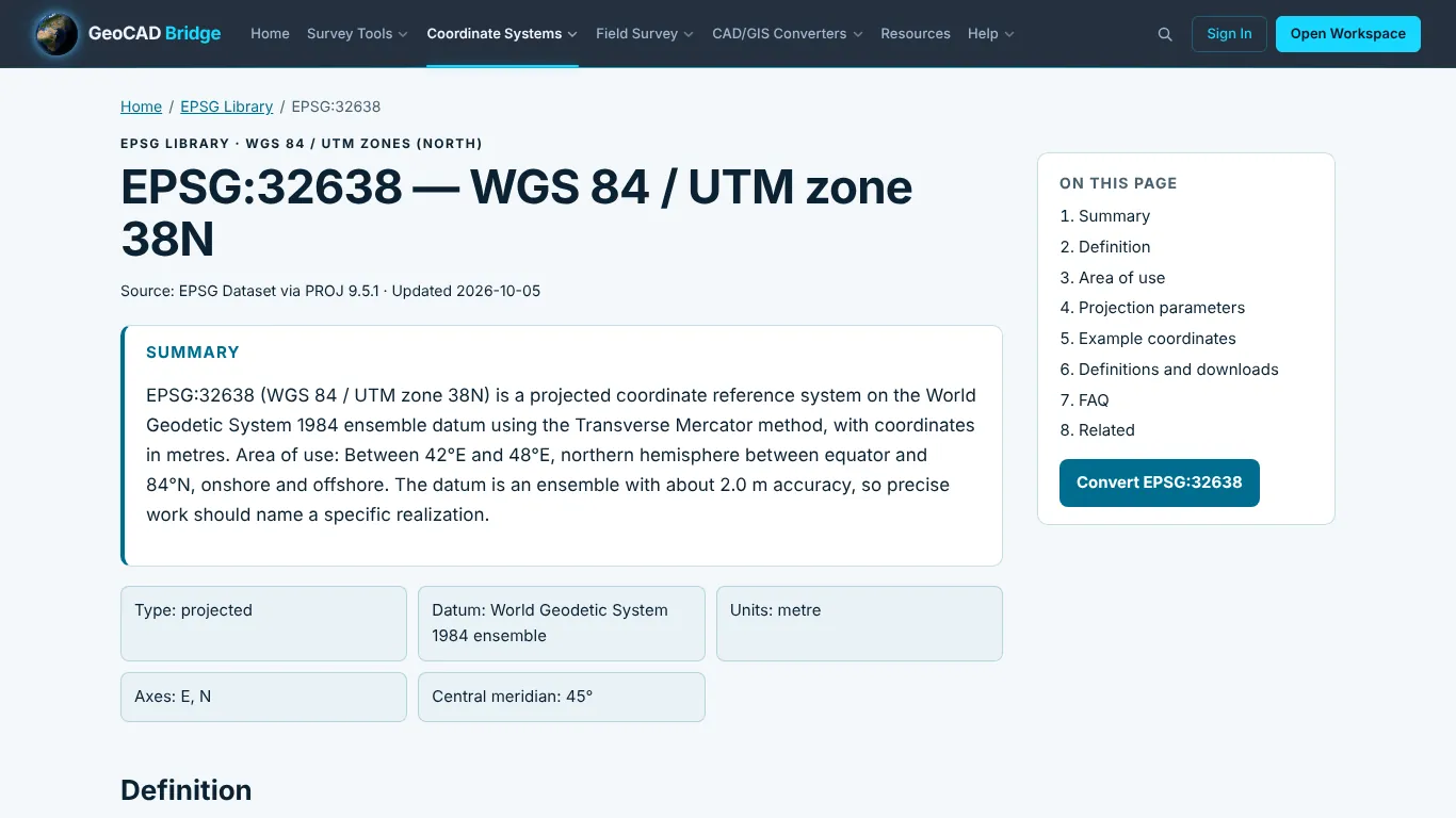
How to find a system. Type an EPSG code, a name (for example Egypt Red Belt), a country or a UTM zone in Search CRS / EPSG, or browse the regional lists. Click a code to open its page, or the converter link next to it.
What each EPSG page contains (227 pages, one per system, address /epsg/<code>/, for example /epsg/32638/):
| Section | Content |
|---|---|
| Summary | Type, datum, units, axes, central meridian and a plain-language description |
| Definition | EPSG code, name, type, datum (with ensemble accuracy), ellipsoid (a and 1/f), prime meridian, projection method, axes, scope, bounding box |
| Area of use | Text description and the list of countries |
| Projection parameters | Every parameter with value and unit (for example latitude/longitude of origin, scale factor 0.9996, false easting 500 000) |
| Example coordinates | A worked conversion computed with PROJ, with the point scale factor and grid convergence, and a link that opens it in the converter |
| Definitions and downloads | PROJ string, the Proj4js definition used by the converter, and downloadable .prj and .wkt files |
| FAQ, Related, References, Cite this page | Nearby and related systems, Knowledge Center articles and tools such as /crs-tools/?crs=<code> and /survey-calculators/#scale |
Using the downloads. The .prj file is the projection file used by Shapefiles, ArcGIS and QGIS: save it next to a Shapefile with the same base name. Example: /epsg/32638/32638.prj. The WKT file contains the full WKT definition. Prefer the EPSG code or WKT2 over a PROJ string, which cannot carry every EPSG detail.
CRS Toolkit /crs-tools/
Three tools in tabs, all running in the browser on 227 systems from the EPSG Dataset (PROJ 9.5.1).
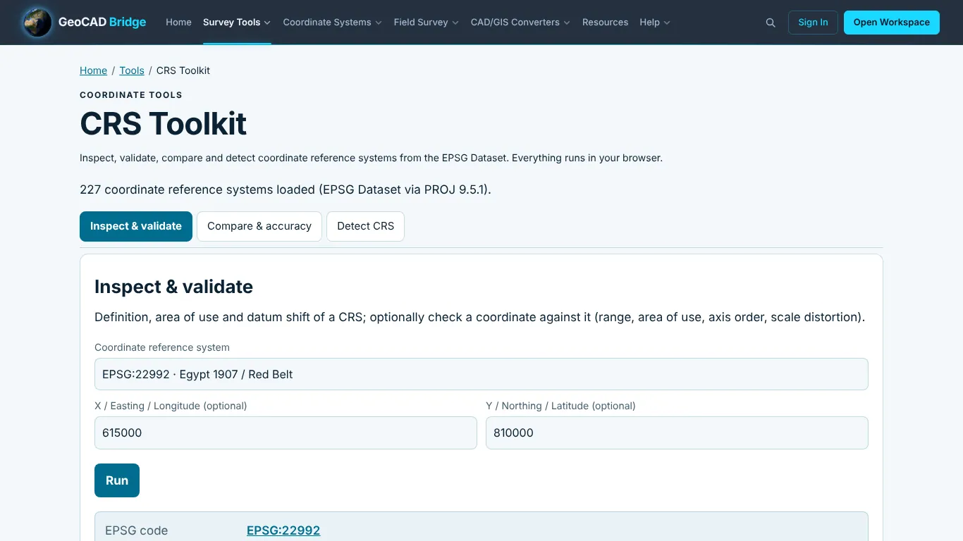
1. Inspect & validate. Enter a Coordinate reference system (code or name) and optionally a coordinate (X / Easting / Longitude, Y / Northing / Latitude), then Run. You get the definition (EPSG code, name, type, datum, ellipsoid, projection method, axes and units, area of use), the datum shift to WGS 84 with its EPSG accuracy, the Proj4js definition and the projection parameters. With a coordinate, the Coordinate check reports whether it is valid, its WGS 84 longitude/latitude, whether it is inside the area of use, and the point scale factor.
Example: CRS 22992 (Egypt 1907 / Red Belt), E 615000, N 810000 → valid, 30°00′00.60″ N 31°00′06.02″ E, inside the area of use, scale factor 1.00000001. The shift to WGS 84 is Egypt 1907 to WGS 84 (1) with an EPSG accuracy of 11 m.
2. Compare & accuracy. Enter CRS A and CRS B and an optional test point. The tool shows the Transformation path and accuracy (the steps and their combined accuracy) and, for the test point, how far it moves if the two systems are confused. Use it before mixing data from two systems.
3. Detect CRS. Paste coordinates of unknown origin, one per line as X, Y (Easting or Longitude, then Northing or Latitude), add an Approximate site location (optional): longitude, latitude, and Run. The result is a ranked list of systems that fit. The site location removes the ambiguity between UTM zones.
Example: paste 652578.355, 2655039.017 and the site 46.5, 24.0. 75 systems place the point inside their area of use; ranked by distance from the site, the first three are EPSG:20438 Ain el Abd / UTM 38N, EPSG:9358 KSA-GRF17 / UTM 38N and EPSG:32638 WGS 84 / UTM 38N. The Same projection, other datum column shows that these three share the projection, so only knowledge of the source datum can separate them.
Country CRS pages
Five reference pages explain the coordinate systems used in the region and give one-click conversion links.
| Page | Address | Main content |
|---|---|---|
| Saudi Arabia | /country-crs/saudi-arabia/ |
UTM zones 37N (EPSG:32637, western and central, including Jeddah, Makkah, Madinah, Riyadh workflows) and 38N (EPSG:32638, eastern); KSA-GRF17 national frame; legacy Ain Al Abd 1970, Aramco frames, GDMS, MTRF-2000 |
| Egypt | /country-crs/egypt/ |
UTM 35N (Western Desert), 36N (central and eastern, Cairo), 37N (Sinai); Egypt 1907 belts; production notes on zone choice |
| UAE | /country-crs/uae/ |
UTM zone 40N and UAE reference data |
| Qatar | /country-crs/qatar/ |
UTM zone 39N, Qatar systems and EPSG codes |
| Gulf Region | /country-crs/gulf/ |
GCC overview and common Gulf survey workflows |
Each page has a Coordinate library box with one button per country (the Gulf page has Saudi Arabia, United Arab Emirates, Qatar, Kuwait, Bahrain and Oman). Click a country to open the library on that country, pick a system, and the page opens Coordinate Transformation with that system as the source. Each page also has Quick Transformations buttons (WGS84 → UTM, UTM → WGS84, Batch Transform and the main zone code), survey standards (coordinate format conventions, datum transformation notes), accuracy notes and related tools. Old addresses such as /saudi-arabia-crs.html redirect to these pages.
Traverse Adjustment /traverse/
Adjusts closed loop, open and link traverses with the Bowditch (compass) rule, the Transit rule or least squares, plots the traverse, and produces reports.
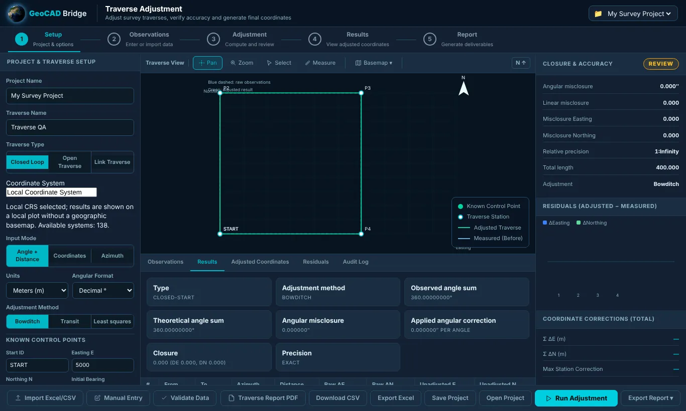
Screen layout
- Step bar: 1 Setup (Project & options) · 2 Observations (Enter or import data) · 3 Adjustment (Compute and review) · 4 Results (View adjusted coordinates) · 5 Report (Generate deliverables).
- Left – Project & Traverse Setup: Project Name, Traverse Name, Traverse Type (Closed Loop, Open Traverse, Link Traverse), Coordinate System (Local, or any of the 138 systems – with a real CRS the traverse is drawn on a basemap), Input Mode (Angle + Distance, Coordinates, Azimuth; the import list also offers RW5), Units (Meters, Feet), Angular Format (Decimal °, DMS as D.MMSS), Adjustment Method (Bowditch, Transit, Least squares, with σ angle in seconds and σ distance in mm + ppm for least squares), and Known Control Points (Start ID, Easting E, Northing N, Initial Bearing, Angle Direction counter-clockwise/clockwise, and for a link traverse Known End E and Known End N).
- Centre – Traverse View with Pan, Zoom, Select, Measure, Basemap and a legend (known control point, traverse station, adjusted traverse, measured before adjustment), and below it the tabs Observations, Results, Adjusted Coordinates, Residuals, Audit Log.
- Right – Closure & Accuracy: angular misclosure, linear misclosure, misclosure in Easting and Northing, relative precision, total length, adjustment method, a residuals chart and the coordinate corrections (Σ ΔE, Σ ΔN, max station correction).
- Bottom bar: Import Excel/CSV, Manual Entry, Validate Data, Traverse Report PDF, Download CSV, Export Excel, Save Project, Open Project, Run Adjustment, Export Report ▾.
Step by step
- Setup. Enter the names, choose the traverse type, input mode, units, angular format and method.
- Known control points. Enter the start station and its coordinates, the initial bearing and the angle direction. For a link traverse also enter the known end point.
- Observations. Type or paste the rows (Point Name, Deg, Min, Sec, Measured Distance; the Decimal Angle column fills itself), or click Upload Excel / CSV / RW5. Load example fills a ready traverse to try the tool. Click Validate Data to catch missing or impossible values.
- Run Adjustment. Read the closure panel: angular misclosure, linear misclosure and precision ratio (for example 1:25 000). Compare them with your specification before accepting.
- Review. Adjusted Coordinates lists the final E/N; Residuals shows the correction at every station; Audit Log records every action. The map shows the measured (blue dashed) and adjusted (green) traverse.
- Report and save. Traverse Report PDF, Download CSV, Export Excel or Export Report ▾. Save Project keeps the whole traverse to reopen later with Open Project.
Templates
- Full input workbook (sheets: Instructions, Project_Settings, Angle_Distance_Input, Coordinate_Input, Control_Points, Code_Lists, and three worked examples: closed loop, connected (link) and open): https://www.geocadbridge.com/downloads/GeoCAD_Bridge_Traverse_Input_Template.xlsx (also on the page: Download Excel Template).
- Angles and distances (CSV): https://www.geocadbridge.com/downloads/Traverse_Angles_Distances_Template.csv
- Observed coordinates (CSV): https://www.geocadbridge.com/downloads/Traverse_Coordinates_Template.csv
- Control points (CSV): https://www.geocadbridge.com/downloads/Traverse_Control_Points_Template.csv
- Simple observation sheet: https://www.geocadbridge.com/downloads/Traverse-Simple.xlsx
- Real-data example workbooks (a closed airport traverse in two parts): https://www.geocadbridge.com/downloads/Jazan-Part1.xlsx, https://www.geocadbridge.com/downloads/Jazan-Part2.xlsx
Worked example. Click Load example, keep Closed Loop, Angle + Distance, Decimal °, Bowditch, then Run Adjustment. The example is a 100 m square starting at START (E 5000, N 5000) with four 90° interior angles. Results: observed angle sum 360°, theoretical sum 360°, angular misclosure 0″, linear misclosure 0.000, precision exact, total length 400.000. Change one distance to 100.02 and run again to see a linear misclosure and how Bowditch distributes it in proportion to leg length.
Common mistakes. A wrong angle direction (clockwise vs counter-clockwise) is the most common cause of a huge misclosure. DMS is typed as D.MMSS: 45°30′15″ is 45.3015. An open traverse has no closing check, so it is computed but cannot be adjusted.
Survey Calculators /survey-calculators/
Seventeen calculators on one page. Above the tabs choose the Angle input format (Decimal degrees or DMS symbols such as 45°30'15", or Packed D.MMSS such as 45.3015) and the number of Decimals (2, 3 or 4). Each tab has a Calculate button; tables can be downloaded as CSV. The Formulas used section at the bottom lists every formula.
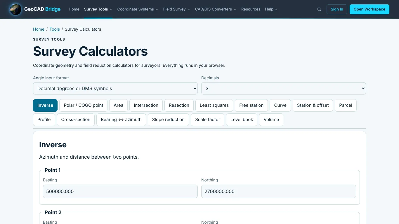
| Tab | Enter | You get |
|---|---|---|
| Inverse | Point 1 and Point 2 (Easting, Northing, optional elevations) | Azimuth 1→2 and back azimuth, quadrant bearing, horizontal distance, ΔE, ΔN (and slope data with elevations) |
| Polar / COGO point | Easting, Northing, Azimuth, Horizontal distance | The new point |
| Area | Points, one per line: Easting, Northing |
Area, perimeter, centroid |
| Intersection | Method: Bearing–bearing, Distance–distance or Angle–angle (forward intersection), two known points, the value at A and at B, and for angle–angle the side (right or left of A→B) | The intersection point(s) |
| Resection | Three known points (A, B, C) and the readings to them | Station coordinates and orientation (Tienstra). Refused near the danger circle or when the readings do not fit |
| Least squares | Control points (fixed), observations (angle, at, backsight, foresight, … and distances), optional approximate coordinates | Adjusted coordinates with σE, σN and error ellipses, residuals with redundancy and w-test; CSV downloads |
| Free station | Station name, direction σ (″), distance σ (m), targets (Point, Easting, Northing, Direction, Distance) | Station coordinates by least squares with residuals |
| Curve | Radius R, deflection angle Δ, direction (right/left), PI chainage, setting-out interval, PI coordinates and back tangent azimuth (optional) | T, L, C, E, M, chainages of PC/PT and a setting-out table with deflections, chords and coordinates (CSV) |
| Station & offset | Start chainage, alignment vertices, and points (Name, Easting, Northing or Name, @chainage, offset) |
Chainage and offset of each point, or the point at a chainage/offset |
| Parcel | Start point and legs (azimuth or quadrant bearing such as N 45 30 00 E, distance) |
Misclosure, precision, area and the Bowditch-closed corners |
| Profile | Rows: Chainage, Ground level, Design level (optional) | Grades and the profile |
| Cross-section | Ground and design sections (Offset, Level per line) |
Cut and fill areas |
| Bearing ↔︎ azimuth | N/S, angle 0–90°, E/W – or an azimuth 0–360° | The other form |
| Slope reduction | Slope distance, zenith angle, instrument and target heights (optional) | Horizontal distance and height difference |
| Scale factor | Projected CRS, latitude, longitude, ellipsoidal height | Point scale factor k, elevation factor, combined scale factor and grid convergence |
| Level book | Start benchmark, closing benchmark (optional), rows: Point, BS, FS, distance from previous | Rise/fall, reduced levels and misclosure distribution |
| Volume | Sections: Chainage (m), Area (m²) | Average-end-area and prismoidal (Simpson) volumes |
Worked examples. Every tab opens with example values, so you can press Calculate straight away and compare with these results:
| Tab | Example input (the page defaults) | Result |
|---|---|---|
| Inverse | P1 E 500 000.000, N 2 700 000.000 · P2 E 500 250.000, N 2 699 900.000 | Azimuth 111°48′05.1″, back azimuth 291°48′05.1″, bearing S 68°11′54.9″ E, distance 269.258, ΔE 250.000, ΔN −100.000 |
| Polar / COGO point | E 500 000, N 2 700 000, azimuth 111°48′05″, distance 269.258 | E 500 250.000, N 2 699 900.000 |
| Area | 0,0 · 100,0 · 100,50 · 0,50 | 5 000.000 m² (0.5 ha, 1.2355 acres), perimeter 300.000, centroid E 50, N 25, counter-clockwise |
| Slope reduction | SD 100.000, zenith 80°00′00″, HI 1.500, HT 1.600 | HD 98.481, vertical component 17.365, height difference 17.265 |
| Scale factor | EPSG:32638, latitude 24.7136, longitude 46.6753, height 600 m | E 669 459.622, N 2 734 271.672, k = 0.99995466, convergence 0°42′02.1″, elevation factor 0.99990583, combined factor 0.99986050 (1 000 m ground = 999.860 m grid) |
| Level book | BM1 = 100.000, closing BM2 = 101.250, rows BM1 / TP1 / TP2 / BM2 | Reduced levels by height of instrument, ΣBS − ΣFS = 1.246, arithmetic check passes, misclosure −4.0 mm distributed by distance (adjusted BM2 = 101.250) |
| Volume | Chainages 0–80 m every 20 m with areas 12.5, 18.2, 22.0, 15.4, 9.8 m² | Average end area 1 335.000 m³, prismoidal (Simpson) 1 338.000 m³ |
| Curve | R 300 m, Δ 40°00′00″ right, PI chainage 1 000, interval 20 m, PI E 501 000 N 2 705 000, back tangent 30° | T 109.191, L 209.440, C 205.212, E 19.253, M 18.092, PC 890.809, PT 1 100.248, forward tangent 70°, setting-out table every 20 m |
| Bearing ↔︎ azimuth | S 30°15′00″ E | Azimuth 149°45′00″, back azimuth 329°45′00″ |
Related articles: azimuths, quadrant bearings, differential leveling, distance reduction, traverse adjustment, UTM (links at the bottom of the page).
Field Visit Survey /field-visit-survey/
The one field page of the site (the former Field Survey Processing page now opens here). A complete site-visit recorder: projects, visits, mapped records, photos, voice notes, measurements, dashboards and reports. All data is stored in this browser until you export it.
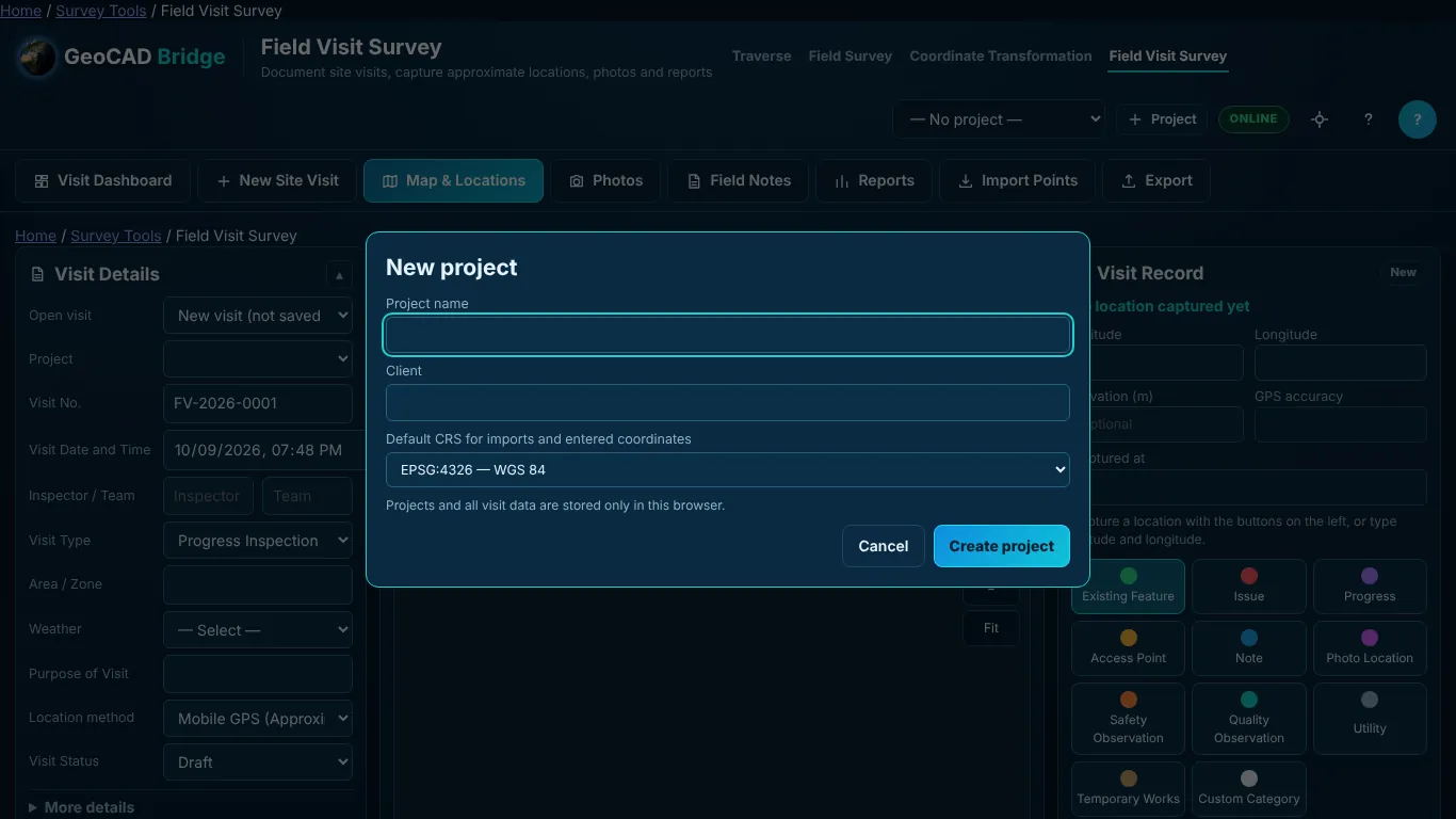
Tabs: Visit Dashboard, New Site Visit, Map & Locations, Photos, Field Notes, Reports, Import Points, Export. Header buttons: Project, Settings, Help.
1. Create a project. Project › New project: Project name, Client and the Default CRS for imports and entered coordinates (chosen from the coordinate library), then Create project.
2. Start a visit. On New Site Visit fill Visit Details: Visit No., date and time, Inspector / Team, Visit Type (Progress Inspection, Existing Conditions Survey, Access Inspection, Issue Investigation, Handover Inspection, Quality Inspection, Safety Observation, Maintenance Inspection, Utility Inspection, General Site Visit, Custom Type), Area / Zone, Weather (Clear, Partly cloudy, Cloudy, Rain, Dust, Windy, Hot, Other), Purpose, Location method (Mobile GPS (Approximate), Manually selected on map, Manually entered coordinates) and Visit Status (Draft, Open, In Progress, Completed, Closed). More details adds Description, Attendees, Contractor, Consultant and Related request / document no. Click Save Visit.
3. Capture records. Use Use Current Mobile Location, Select Location on Map (then Confirm location) or Enter Coordinates. In Visit Record choose a category (Existing Feature, Issue, Progress, Access Point, Note, Photo Location, Safety Observation, Quality Observation, Utility, Temporary Works, Custom Category), a Title, Status (Open, In Progress, Resolved, Closed, For Review, Monitoring, Information Only), Description / Observations, Recommendation / required action, Responsible party, Due date, photos (Take Photo, Upload Photos), Add Voice Note, Include in Final Report, then Save Visit Record. New record / Delete record manage records.
4. Map tools. Search location or point ID, basemap (None, Streets, Satellite, Hybrid, Terrain, Light, Dark), Labels, Pan, Select, Identify, Fit, Show All Points, Measure Between Points, Clear Measurement, Zoom to Points. Table tabs: Visit Records, Uploaded Points, Photos, Notes, Measurements, Activity Log; row actions: Add Point, Remove Selected, Hide Selected, Copy Coordinates, Add to Visit, Add to Report, Export Selected.
5. Import points. On Import Points drop a file (Excel .xlsx/.xls, CSV, KML, KMZ, GeoJSON) and use Open import wizard… to map columns and choose the CRS; nothing is assumed. Templates: Download CSV template https://www.geocadbridge.com/downloads/Field_Visit_Points_Template.csv and Download Excel template https://www.geocadbridge.com/downloads/Field_Visit_Points_Template.xlsx (the Excel file has an Instructions sheet).
6. Dashboard. Visits by status, records by category, visits by area, recent visits and a map of visits.
7. Report. Reports builds the report for the current visit from records marked Include in Final Report: PDF report (print → Save as PDF) or Download report (HTML).
8. Export and back up. Export saves selected records as CSV, Excel, GeoJSON, KML or KMZ, and the complete visit package (.zip). Reopen an exported visit package with Choose a visit package (.zip). Export the package regularly: clearing browser data deletes the visits.
Accuracy. Mobile GPS locations are approximate and must not be used for setting-out, legal boundaries, construction control or survey control.
File converter pages
Six one-page converters change a file from one format to another in the browser. They share one interface: a compact header with the page title, a Coordinates button showing the current CRS (for example EPSG:4326), استيراد / Import and تصدير / Export buttons, a full-size map with a basemap list, and a guide below the map.
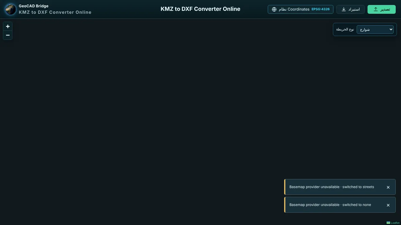
| Converter | Address | Input | Output | Typical use |
|---|---|---|---|---|
| DXF to KMZ | /export-dxf-to-kmz/ |
DXF (points, polylines, lightweight polylines, polygons) | KMZ / KML in WGS 84 | Review CAD linework on imagery, share with non-CAD users |
| KMZ to DXF | /kmz-to-dxf/ |
KMZ / KML vector placemarks | DXF in a projected CRS | Turn a Google Earth boundary or route into CAD linework |
| SHP to DXF | /shp-to-dxf/ |
Zipped Shapefile (SHP, SHX, DBF, PRJ) | DXF | Use GIS parcels, corridors or utilities in CAD |
| SHP to KMZ | /shp-to-kmz/ |
Zipped Shapefile | KMZ / KML | Share GIS layers as Google Earth overlays |
| CSV Point to KMZ | /csv-point-to-kmz/ |
CSV points (name plus longitude/latitude or easting/northing; elevation and description optional) | KMZ / KML | Control, stakeout lists, boreholes, assets |
| GeoJSON to KMZ | /geojson-to-kmz/ |
GeoJSON (Point … MultiPolygon, FeatureCollection) | KMZ / KML | Web-map or API data in Google Earth |
Workflow (same on every converter)
- Click Coordinates and choose the source CRS. Shapefiles carry it in the PRJ; DXF and CSV usually do not, so you must choose it. KML/KMZ and GeoJSON are WGS 84.
- Click Import and choose the file.
- Inspect the features on the map and the attribute preview. If they land in the sea or near 0,0 the source CRS is wrong.
- Click Export, choose the format (DXF, KML/KMZ, Shapefile ZIP, GeoJSON, CSV Points, Excel), the Scope (entire project, active layer or selected features) and the Output CRS, and download. KML/KMZ is always written in WGS 84; DXF is written in the projected CRS your drawing uses.
The converter pages run on the same engine as the Workspace and use the same import and export dialogs (Part 3). If the data needs editing before export (deleting features, changing attributes, reprojecting, merging layers), open it in the Workspace instead.
Example (CSV points in UTM to KMZ). On /csv-point-to-kmz/ set Coordinates to EPSG:32637, import a CSV with Point,Easting,Northing,Elevation, check the points on the map, then Export › KMZ. The KMZ is written in WGS 84 for Google Earth.
Common mistakes. Uploading only the .shp without .shx/.dbf/.prj; leaving the source CRS on WGS 84 when the CSV contains UTM values; exporting geographic degrees into a CAD drawing that expects metres (the data lands near 0,0); expecting raster image overlays inside a KMZ to become DXF. DWG is not read: save it as DXF in your CAD program.
Knowledge Center /knowledge/
Reference articles for surveyors, geodesists, GIS analysts and CAD engineers. Each full article has a summary, the theory, a worked example with real (computed) numbers, common mistakes, an FAQ and links to the tool that does the calculation.
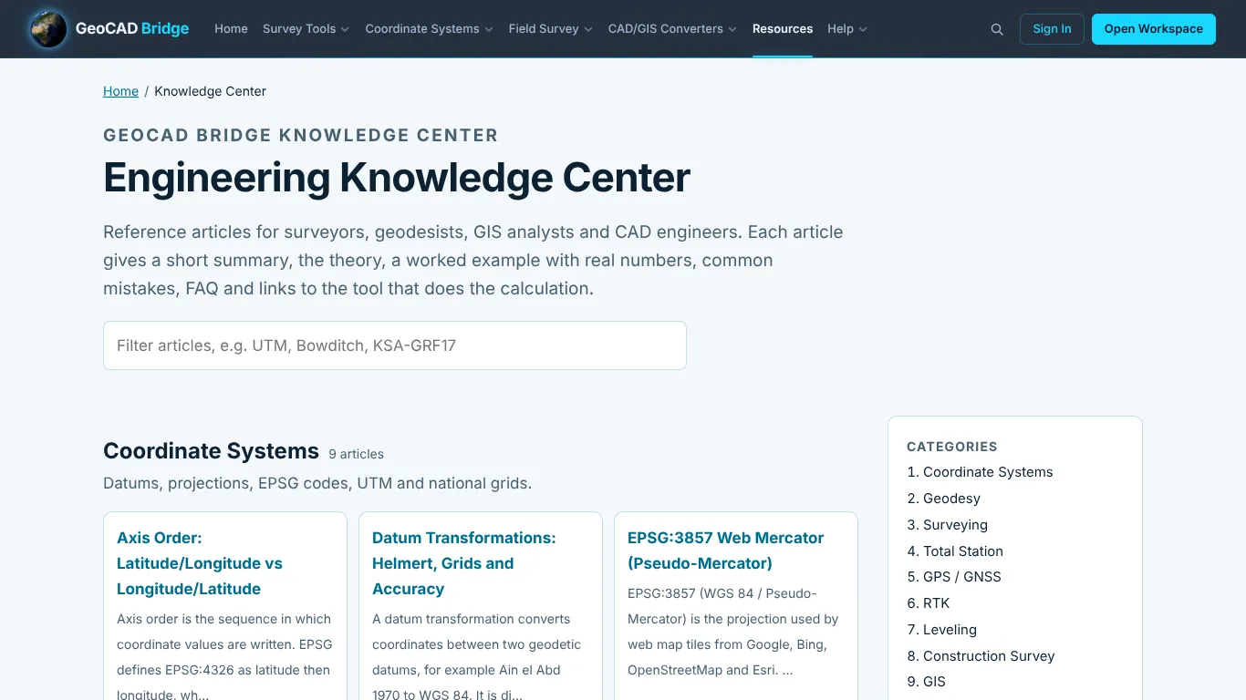
How to use it. Type in Search articles or open a category: Coordinate Systems, Geodesy, Surveying, Total Station, GPS / GNSS, RTK, Leveling, Construction Survey, GIS, Mapping, CAD, File Conversion, Country Coordinate Systems, and the Glossary. Each article ends with Related tools and articles, References and Cite this page.
Full articles
| Topic | Address |
|---|---|
| Axis Order: Latitude/Longitude vs Longitude/Latitude | /knowledge/coordinate-systems-axis-order/ |
| Datum Transformations: Helmert, Grids and Accuracy | /knowledge/coordinate-systems-datum-transformations/ |
| Egypt 1907 Datum and the Egyptian Belts | /knowledge/coordinate-systems-egypt-1907/ |
| EPSG:3857 Web Mercator | /knowledge/coordinate-systems-epsg-3857/ |
| EPSG:4326 WGS 84 Latitude/Longitude | /knowledge/coordinate-systems-epsg-4326/ |
| Grid Shift Transformations (NTv2, NADCON, GeoTIFF) | /knowledge/coordinate-systems-grid-shifts/ |
| KSA-GRF17 Saudi Arabia Geodetic Reference Frame | /knowledge/coordinate-systems-ksa-grf17/ |
| Ain el Abd 1970 Datum (Saudi Arabia) | /knowledge/coordinate-systems-saudi-ain-al-abd/ |
| Transverse Mercator Projection | /knowledge/coordinate-systems-transverse-mercator/ |
| UTM Zones: Find the Right Zone and EPSG Code | /knowledge/coordinate-systems-utm-zones/ |
| UTM Coordinate System Explained | /knowledge/coordinate-systems-utm/ |
| WGS 84: World Geodetic System 1984 | /knowledge/coordinate-systems-wgs84/ |
| Angular Misclosure in Traverse Surveys | /knowledge/survey-angular-misclosure/ |
| Azimuths: Grid, True and Magnetic North | /knowledge/survey-azimuths/ |
| Quadrant Bearings in Surveying | /knowledge/survey-bearings/ |
| Bowditch Rule (Compass Rule) | /knowledge/survey-bowditch-rule/ |
| Closed Traverse: Loop and Link | /knowledge/survey-closed-traverse/ |
| Distance Reduction: Slope to Horizontal to Grid | /knowledge/survey-distance-reduction/ |
| GPS / GNSS Surveying Methods Compared | /knowledge/survey-gps-survey/ |
| Least Squares Adjustment for Surveyors | /knowledge/survey-least-squares/ |
| Differential Leveling: Height of Instrument Method | /knowledge/survey-leveling/ |
| Link Traverse (Connecting Traverse) | /knowledge/survey-link-traverse/ |
| Open Traverse: Uses, Risks and Checks | /knowledge/survey-open-traverse/ |
| Traverse Precision Ratio | /knowledge/survey-precision-ratio/ |
| RTK GNSS Surveying: Accuracy and Quality Control | /knowledge/survey-rtk-survey/ |
| Construction Stakeout (Setting Out) | /knowledge/survey-stakeout/ |
| Total Station Survey Workflow | /knowledge/survey-total-station-workflow/ |
| Transit Rule Traverse Adjustment | /knowledge/survey-transit-rule/ |
| Traverse Adjustment: Complete Guide for Surveyors | /knowledge/survey-traverse-adjustment/ |
Short reference pages. In addition, 531 short topic pages cover coordinate topics (405), country systems (40), CAD (30), GIS (30), survey (30) and converter formats (25, for example /knowledge/converters-dxf-to-kml/, /knowledge/converters-csv-to-shp/). They are reachable from the category lists and are kept out of search engines until a full article replaces them.
Resources & Templates /resources/
Downloads for every tool, with filters.
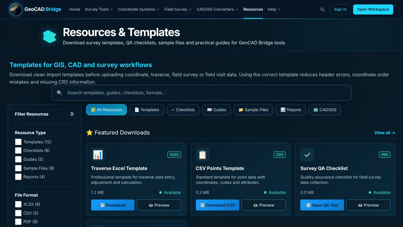
Filters: Resource Type (Templates, Checklists, Guides, Sample Files, Reports), File Format (XLSX, CSV, PDF, DOCX, KML/KMZ, DXF, GeoJSON), Topic (Coordinate Systems, Field Survey, Data Processing, CAD/GIS, Reporting) and Status. Category buttons: All Resources, Templates, Checklists, Guides, Sample Files, Reports, CAD/GIS.
Sections and what each button does
| Card | Button | Goes to |
|---|---|---|
| Traverse Excel Template | Download | /downloads/GeoCAD_Bridge_Traverse_Input_Template.xlsx |
| CSV Points Template | Download CSV | /downloads/Field_Visit_Points_Template.csv |
| Survey QA Checklist | Open QA Tool | /field-visit-survey/ |
| Field Visit Report Template | Download | /downloads/Field_Visit_Points_Template.xlsx (the visit report itself is produced on /field-visit-survey/ › Reports) |
| Coordinate Systems Guide | Open Guide | /coordinate-systems/ |
| EPSG Quick Reference | Open EPSG Finder | /coordinate-transformation/?mode=epsg |
| Field Survey Processing Guide | Open Guide | /field-visit-survey/ |
| KML/KMZ Export Guide | Open CAD/GIS Tools | /workspace/ |
| Sample Survey Points CSV | Download CSV | /downloads/Field_Visit_Points_Template.csv |
| Sample KML/KMZ, Sample DXF, Sample GeoJSON | Open KML / DXF / GeoJSON Tools | /workspace/ |
The Recommended Resource Pack shows the order: Start with Sample Template → Choose CRS Guide → Validate QA Checklist → Export Report Template. The complete list of downloadable files is in Appendix A.
Help Center /help/
Bilingual (English + Arabic) guides. Use the EN + ع / English / العربية switch at the top of each help page.
| Page | Address | Content |
|---|---|---|
| Help Center | /help/ |
Index of all guides |
| How to use Workspace | /help/workspace/ |
Open/create a project, set the CRS, import, layers, draw and edit, measure and analyse, export, save |
| How to use Traverse Adjustment | /help/traverse/ |
Setup, control points, observations, run, review, report |
| How to use Coordinate Transformation | /help/coordinate-transform/ |
Source and target CRS, entering coordinates, transform, batch, copy/export |
| How to use Field Survey | /help/field-survey/ |
Project and visit, location, records, import, comparison, report |
| How to use File Converters | /help/file-converters/ |
Source CRS, import, inspect, export |
| How to use EPSG Reference | /help/epsg-reference/ |
Search, read a CRS page, download .prj/.wkt, use in a conversion |
| Support | /help/support/ |
Contact form (Name, Email, Subject, Message → Send message opens your e-mail program) |
| About | /help/about/ |
Version 2.1, the technology used (Leaflet, Proj4js, EPSG Dataset, Turf.js, SheetJS, JSZip/shpjs/shp-write, dxf-parser/togeojson, Supabase) |
| Keyboard Shortcuts | /help/shortcuts/ |
All shortcuts (Appendix B) |
| What’s New | /help/whats-new/ |
Release notes for version 2.1 |
Writing to support. Say which tool and page you used, give the EPSG code and file format if the problem is about data, and attach a sample file or screenshot after your e-mail program opens.
Arabic pages /ar/
Fourteen tools have a full Arabic interface (right-to-left) under /ar/. Use the العربية link on the English page or open the address directly:
| Arabic page | Address |
|---|---|
| تحويل الإحداثيات | /ar/coordinate-transformation/ |
| محول الإحداثيات | /ar/coordinate-converter/ |
| المحول الجماعي | /ar/batch-coordinate-converter/ |
| WGS84 إلى UTM | /ar/wgs84-to-utm/ |
| UTM إلى WGS84 | /ar/utm-to-wgs84/ |
| خط العرض والطول إلى UTM | /ar/lat-long-to-utm/ |
| UTM إلى خط العرض والطول | /ar/utm-to-lat-long/ |
| محول EPSG | /ar/epsg-converter/ |
| محول CRS | /ar/crs-converter/ |
| محول إحداثيات السعودية | /ar/saudi-arabia-coordinate-converter/ |
| محول إحداثيات مصر | /ar/egypt-coordinate-converter/ |
| مكتبة EPSG | /ar/epsg/ |
| زيارة موقع ميدانية | /ar/field-visit-survey/ |
| ضبط الترافيرس | /ar/traverse/ |
The Arabic pages work exactly like the English ones. Exported files keep English field names so they open the same way in every program. The Workspace switches language with its العربية button (Part 3).
Admin page
/admin.html is the owner’s administration page for the file library (sign-in with the owner account). It is not linked from the site and is not needed by users.
Part 3 · The Workspace /workspace/
The Workspace is a complete CAD · GIS · survey program that runs in the browser. You open it from the Workspace link in the navigation bar or at https://www.geocadbridge.com/workspace/. Nothing is installed and no account is needed. Your data stays in your browser until you save a project file or export results.
This part explains the Workspace from the first screen to the last command:
- The screen layout and every area on it.
- Projects: create, open, save, recover.
- Coordinate systems: project CRS, layer CRS, the coordinate library, Reproject Layer.
- Importing data and exporting results.
- Layers, the Inspector, selection and editing.
- The CAD command line.
- A tab-by-tab reference of the ribbon tabs and every command.
- The survey panels in depth (Total Station, Static GNSS, Area & Volume, Surfaces, Grading, Traverse Correction, Bridge, reports).
- Worked examples from start to finish.
The screen layout
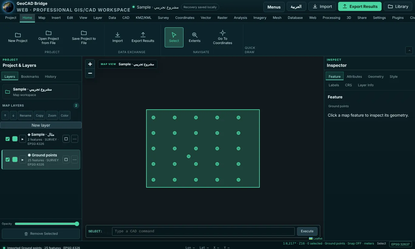
| Area | Where | What it does |
|---|---|---|
| Header | Top row | Project name and save state (Recovery saved locally / Unsaved), and the buttons Menus, العربية, Import, Export Results and Library. |
| Ribbon | Under the header | 25 tabs (Project … Help). Each tab holds groups of commands; the group name is written under it. The ⌃ button at the right collapses the ribbon. |
| Project & Layers | Left | Three tabs: Layers, Bookmarks, History. |
| Map view | Centre | The drawing and map area, with + / − zoom and the map title. |
| CAD command line | Bottom of the map | Type commands and coordinates (see The CAD command line). |
| Inspector | Right | Seven tabs: Feature, Attributes, Geometry, Style, Labels, CRS, Layer Info. |
| Status bar | Bottom | The last message, cursor coordinates (Lon, Lat, X, Y), map scale, zoom, number selected, active layer, snap state, units, current tool and the project EPSG code. |
Header buttons
- Menus switches the ribbon to a classic menu bar (Project, Map, Insert, Analysis, Imagery, Share, Edit, View, Layer, Data, CAD, KMZ/KML, Survey, Coordinates, Vector, Raster, Database, Web, Mesh, Processing, 3D, Settings, Plugins, Help…). Each menu drops down the same commands as the ribbon tab of the same name. The button then reads Ribbon; click it to return.
- العربية switches the whole Workspace interface to Arabic (right-to-left). Click English to switch back. Data and file contents are not changed.
- Import opens the Import Data dialog (see Importing data).
- Export Results opens the Export dialog (see Exporting results).
- Library opens the File Library: ready-to-use survey, GIS and CAD resources, filtered by All categories, Survey, GIS, CAD, Guides. Visitors can download files; uploading is reserved for the site owner.
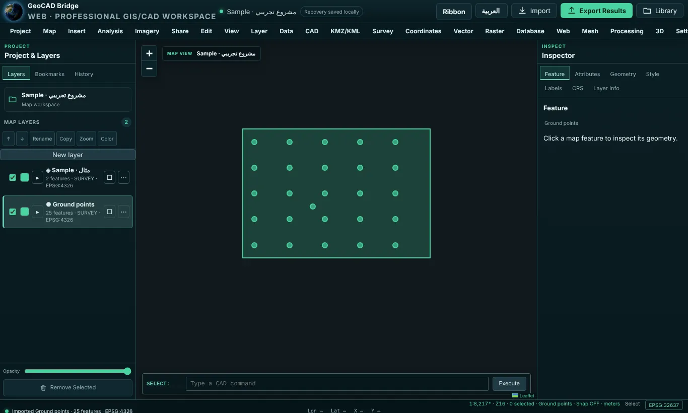
The Layers panel
The Layers tab lists the project’s map layers, top layer first. The number next to MAP LAYERS is the layer count.
- ↑ / ↓ move the selected layer up or down in the drawing order (you can also drag a row).
- Rename renames the selected layer (or double-click its name, or press F2).
- Copy duplicates the layer. Zoom zooms to the layer. Color changes the layer colour.
- New layer creates an empty layer to draw in or paste into.
- Each row has: a visibility checkbox, a colour swatch, ▸ to expand details (geometry types, opacity, labels on/off, locked/editable), the layer name with its feature count, source format and source CRS, a lock button □ (Lock geometry and attributes; locked layers show ▣ and cannot be edited), and ⋯ for layer actions.
- ⋯ / right-click menu: Zoom to Layer, Rename, Duplicate, Style / Properties, Labels, Export Layer, Bridge to AutoCAD / Civil 3D / QGIS / Trimble…, Delete.
- Opacity slider sets the transparency of the selected layer. Remove Selected deletes the selected layer (you are asked to confirm).
Clicking a row makes it the active layer. New features are drawn into the active layer, and many commands work on it.
The Bookmarks tab lists saved map views (create them with View › Locations › Add Bookmark). The History tab lists the actions done in the session.
The Inspector
The Inspector shows details of the selected feature or, when nothing is selected, of the active layer.
| Tab | Shows |
|---|---|
| Feature | Number selected, Feature ID, Layer, Type. For a point: label, E/X and N/Y in the project CRS, Z, latitude, longitude, UTM zone, project CRS and (for UTM projects) the approximate grid scale factor. For a line or polygon: length or perimeter and area (spherical metres). Zoom to selection. |
| Attributes | Attribute table button, the attribute list of the selected feature and Edit attributes. |
| Geometry | The same values plus the full geometry as GeoJSON text and Copy geometry. |
| Style | Style & transparency (opens the layer properties). |
| Labels | Configure labels (choose the label field) and Toggle labels. |
| CRS | Source CRS of the layer, project CRS, Geometry storage: WGS84 (EPSG:4326), Vertical datum: Not transformed, and Choose project CRS. |
| Layer Info | Name, Source, Features, Source CRS, Geometry types, Editing (Locked/Unlocked), Opacity, and Layer properties. |
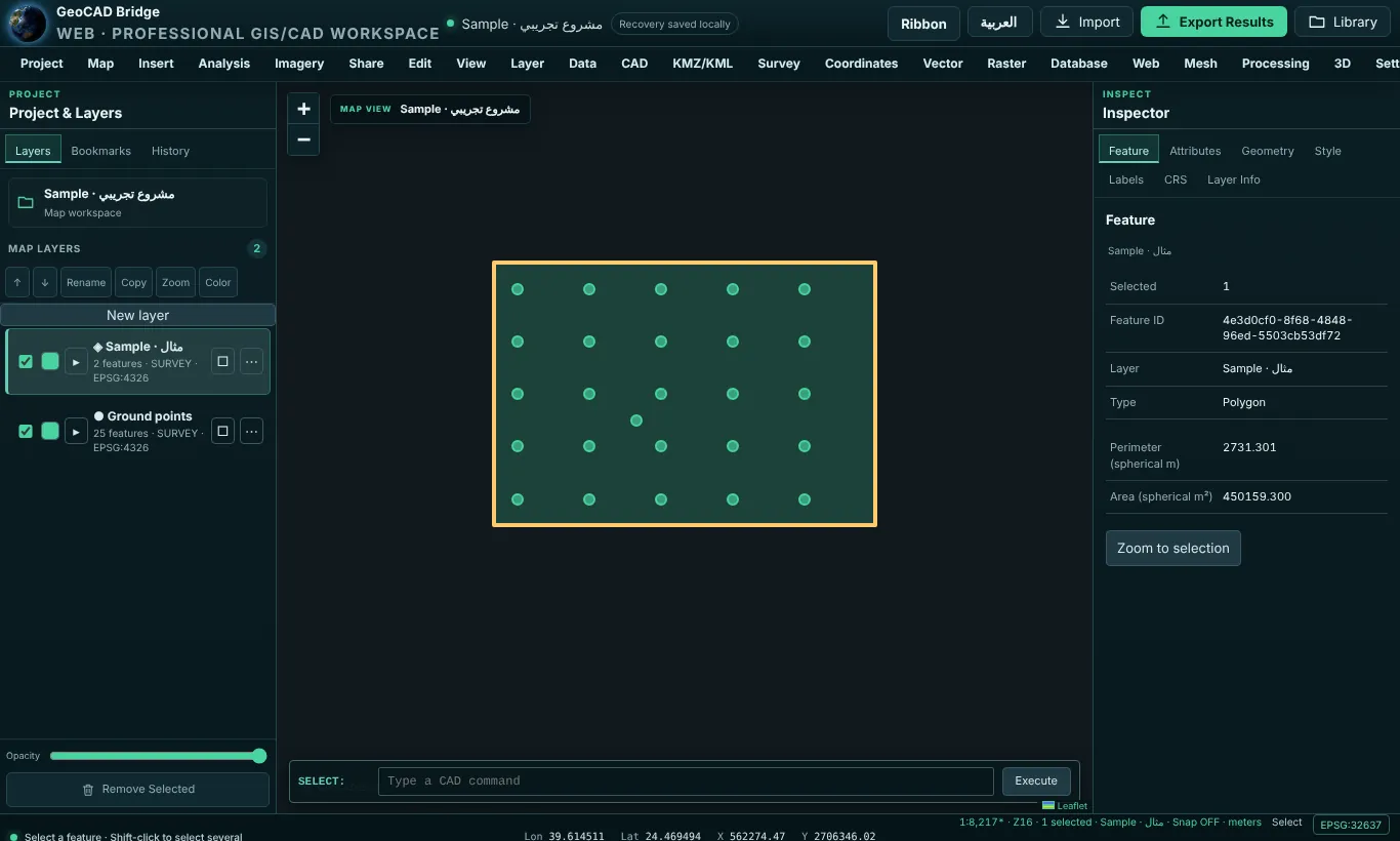
Good to know. All geometry is stored internally as WGS 84 longitude/latitude. The project CRS controls how coordinates are displayed, entered, measured on the grid and exported. Changing the project CRS never moves your data.
The status bar
From left to right: the last message (for example Imported Ground points · 25 features), cursor Lon / Lat / X / Y, the approximate map scale (for example 1:8,217*, at 96 pixels per inch), zoom level, N selected, the active layer, Snap ON/OFF, report units, the current tool, and the project EPSG code. Click the EPSG box to open the coordinate library.
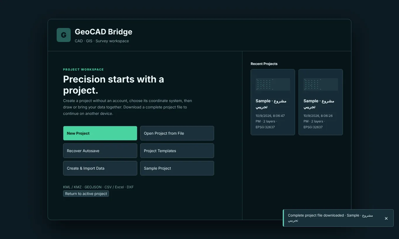
Projects
The start screen (Project Manager)
When no project is open, the Workspace shows the Project Manager.
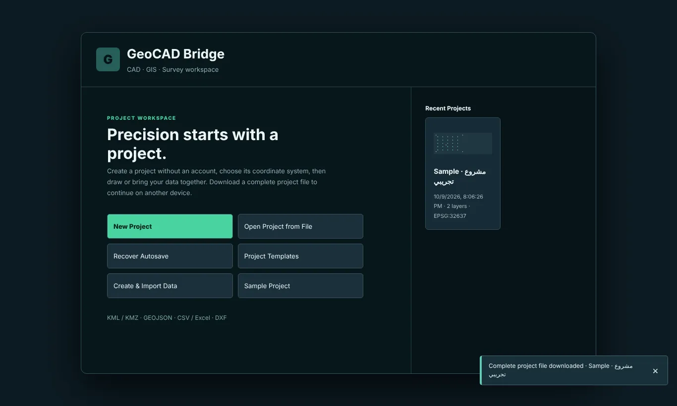
| Button | What it does |
|---|---|
| New Project | Creates an empty project. You name it and choose its coordinate system. |
| Open Project from File | Opens a .gcbproject file you saved earlier (legacy GeoCAD project JSON is accepted too). The file is checked for integrity before it loads. |
| Recover Autosave | Restores the temporary recovery copy that this browser keeps of the last project. |
| Project Templates / UTM 37N Project | Creates a project from a template with real layers, fields and validation rules: Building Survey (building outlines and entrances with field-review attributes) or Utility Inventory (manholes and utility lines with condition and dimension fields). |
| Create & Import Data | Creates a project and opens the import dialog straight away. |
| Sample Project | Creates a ready project in EPSG:32637 with a sample point and polygon to practise on. |
| Recent Projects | Cards of recent projects in this browser (name, date, number of layers, EPSG). Click one to reopen it. |
The note at the bottom lists the main formats you can bring in: KML / KMZ · GeoJSON · CSV / Excel · DXF.
Working without an account
The Work without an account message explains the rule that matters most: the browser only keeps a temporary recovery copy. To keep your work, use Save Project to File and download the .gcbproject file. To continue later or on another computer, use Open Project from File. Files made with Export Results (Excel, KML…) are for sharing data and are not a complete project backup.
What the project file contains
Save Project to File downloads a versioned, integrity-checked .gcbproject file with: project metadata, layer order, visibility and style, feature geometry and attributes, CRS definitions, map view, units, bookmarks and the last QA/QC report summary (from Share › Reports › Supported Formats).
Project commands
- Save / Save Project to File (Ctrl+S): downloads the complete project file.
- Save As / Save Copy (Ctrl+Shift+S): asks for a new project name and downloads a copy under that name.
- Open Project (Ctrl+O): choose a
.gcbprojectfile. - Recover Autosave: restores the temporary copy this browser keeps of the last project.
- Close Project: returns to the Project Manager. If there are unsaved changes you are asked first (Download a saved copy first if you need these changes).
- Project Properties: Name, Location, Description, Report units.
- Project Units: meters or feet for the survey measurement report. Grid calculations stay in metres; coordinate units follow the CRS.
- Project Statistics: a table of every layer with its feature count and CRS.
Coordinate systems in the Workspace
There are two kinds of CRS:
- The project CRS is the grid you work in. Coordinates you type, measurements on the grid, the status-bar X/Y, the Inspector E/N and most exports use it. It is shown in the status bar (for example EPSG:32637).
- Each layer has a source CRS: the system its file came in. It is detected on import and shown in the layer row and the Inspector’s CRS tab.
Choosing a coordinate system (the coordinate library)
Open the coordinate library with Project › Configuration › Project CRS, Coordinates › CRS library › Set Project CRS, the Coordinate library… button in the ribbon, the system shown in the status bar, or Choose project CRS in the Inspector. The New project window has the same button, so the project starts in the right grid.
- Choose a Country / category, or search by code, description, country or EPSG number.
- Click a system to see its projection, datum, unit, EPSG equivalent and datum shift.
- Click OK. The project CRS changes and the button shows the new system.
The chapter The coordinate library in Part 2 describes the window in full.
Reproject Layer (convert a layer to another system)
Analysis › Data management › Reproject Layer (also Raster › Projections › Warp Reproject) converts a whole layer, the way desktop GIS programs do.
- Choose the Layer.
- Choose the Output coordinate system from the coordinate library.
- Click OK. A copy of the layer is added in the chosen system, named for example Points · UTM84-38N. The original layer stays as it is.
Related CRS commands
- Set Layer CRS (Layer tab) tells the Workspace which system a layer’s coordinates are really in, when detection was wrong.
- Set Project CRS from Layer uses the selected layer’s source CRS as the project CRS.
- Validate CRS confirms the project CRS, for example CRS valid: EPSG:32637 · WGS 84 / UTM zone 37N · Madinah.
- Extract Projection shows the projection parameters of the project CRS in a table (CSV download).
- Axis Order Check lists each layer with its source CRS, vertex count and extent (west, south, east, north) and a Result. Use it when points land in the wrong country: it reveals swapped latitude/longitude or Easting/Northing.
- Custom Projections (Settings) opens the coordinate library.
Importing data
Open the import dialog with Import in the header, Home › Import, Project › Import Data, Data › Import Dataset, Layer › Add Layer, Map › Add Data or Insert › Import GIS / CAD.
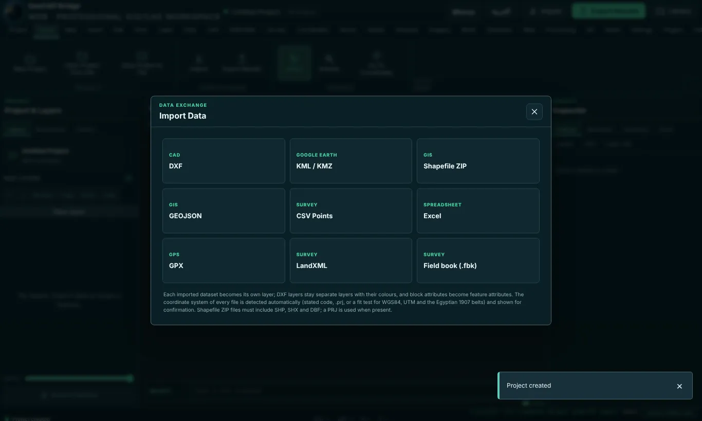
| Card | Files | Notes |
|---|---|---|
| CAD · DXF | .dxf |
DXF layers stay separate layers with their colours; block attributes become feature attributes. |
| Google Earth · KML / KMZ | .kml, .kmz |
Always WGS 84. |
| GIS · Shapefile ZIP | .zip |
Must contain SHP, SHX and DBF; a PRJ is used when present. |
| GIS · GeoJSON | .geojson, .json |
WGS 84. |
| Survey · CSV Points | .csv, .txt |
Point lists with E, N, Z or longitude, latitude. See the import templates. |
| Spreadsheet · Excel | .xlsx, .xls |
First sheet with a header row. |
| GPS · GPX | .gpx |
Waypoints, routes and tracks. |
| Survey · LandXML | .xml |
LandXML 1.2 points and surfaces. |
| Survey · Field book (.fbk) | .fbk, .txt |
Survey field book: points, codes, descriptions and figures (see below). |
| CAD · DWG | — | Not read directly. In AutoCAD use DXFOUT (Save As DXF), then import the DXF. |
What happens on import
- You choose the file. Each dataset becomes its own layer.
- The coordinate system is detected automatically: from a stated code, from the
.prj, or by a fit test for WGS 84, UTM and the Egyptian 1907 belts. It is shown for confirmation; change it if it is wrong. - The layer is added, drawn and zoomed to. The status bar reports, for example, Imported Ground points · 25 features · EPSG:4326.
CSV templates. Help › Reference › Import Templates shows the column names for each workflow and downloads four ready CSV files: survey-points.csv (Point, Easting, Northing, Elevation, Description, Code, Layer, CRS), traverse-coordinates.csv (Point, Easting, Northing, Elevation), traverse-observations.csv (Point, Azimuth, Distance, DeltaElevation) and geographic-points.csv (Name, Longitude, Latitude, Elevation, Description). The first row is the header, use a decimal point, and save CSV as UTF-8 so Arabic text survives.
Example survey-points.csv:
Point,Easting,Northing,Elevation,Description,Code,Layer,CRS
P-101,562599.000,2703054.000,619.250,Control point,CP,Survey Points,EPSG:32637
Import Excel (Data, Insert tabs) opens the file chooser for an .xlsx workbook directly.
Opening a field book (.fbk)
A field book is the text file a total station job is exported to. Open it with Import › Field book (.fbk), Survey › Field data › Field Book (.fbk) or the Menus list.
- Choose the
.fbkfile. - Confirm the coordinate system. It is detected from the coordinates and can be changed with the coordinate library.
- Two layers are added, grouped under the file name:
- Points: each point with its number, code (the first word of the description), description, elevation and type (control, station or shot).
- Figures: the lines recorded between BEG and END. A figure ended with CLOSE becomes a polygon.
- The status bar reports the count, for example Field book site.fbk: 11 points, 2 figures, 1 setups. Lines that could not be read are listed in a notice; the rest of the file is still imported.
The reader understands known points (NE, NEZ, NE SS, LAT LONG), setups (STN with instrument height, BS with circle reading, AZ, B), shots (AD, DD, ZD, BD, F1, F2, each with VA or VD), PRISM, SF, UNITS (metre or foot; DMS, decimal degrees, grads, mils, radians), ANGLES and VERT ANGLE. Angles are read as DDD.MMSS, and vertical angles as zenith angles, unless the file says otherwise. Curves in figures are drawn as straight segments.
Example:
NEZ 1 2700000.000 500000.000 600.000 "CP1 control"
NE 2 2700100.000 500000.000 "CP2"
PRISM 1.500
STN 1 1.500
BS 2
BEG EP
AD VA 3 90.0000 50.000 90.0000 "EP edge"
AD VA 4 180.0000 50.000 84.1720 "EP edge"
END
Point 3 lands 50 m east of point 1 and point 4 about 49.75 m south of it, both on the line EP.
Exporting results
Open the export dialog with Export Results in the header or any Export command (Export Data, Export Dataset, Export Layer, Export Points, Export DXF, Export KML/KMZ, Export Map…).
- Scope: Entire project (including hidden layers), Active layer or Selected features.
- Output CRS: for example EPSG:4326 · WGS 84, EPSG:32637 · WGS 84 / UTM zone 37N, EPSG:9358 · KSA-GRF17 / UTM zone 38N. The line under it tells you what will happen, for example Same coordinate system: coordinates are written unchanged, or that a transformation will be applied.
- Click a format:
| Button | File | CRS used |
|---|---|---|
| GIS · GEOJSON | .geojson |
WGS 84 |
| Google Earth · KML | .kml |
WGS 84 |
| Google Earth · KMZ | .kmz |
WGS 84 |
| GIS · Shapefile ZIP | .zip (SHP, SHX, DBF, PRJ) |
Output CRS (WGS 84, any UTM zone or any EPSG Library system with a .prj) |
| CAD · DXF | .dxf |
Output CRS |
| Survey · CSV | .csv with all attributes |
Output CRS |
| Survey · CSV · Point, X, Y, Z | .csv |
Output CRS |
| Civil 3D · TBC · PNEZD points | .csv Point, Northing, Easting, Z, Description |
Output CRS |
| Spreadsheet · Excel | .xlsx |
Output CRS |
| GPS · GPX | .gpx |
WGS 84 |
| Survey · LandXML | .xml (LandXML 1.2, opens in Civil 3D and Trimble Business Center) |
Output CRS |
| CAD · DWG | — | Requires a DWG engine (not available) |
DBF limits may shorten Shapefile field names or long text. Export Excel writes GCB_* columns that keep style values; spreadsheets do not draw map styles.
Selecting, drawing and editing
- Select (Home, Map or Edit tab): click a feature; Shift-click adds more. Clear Selection empties it. F zooms to the selection.
- Draw a feature with Point, Polyline, Polygon, Rectangle, Circle, 3-Point Arc, Ellipse, Freehand or Construction Line (CAD tab, Insert › Create features, or Edit › Add Polygon Feature). The status bar guides you, for example Polyline · click or enter coordinates · Enter finishes · Esc cancels.
- Finish (Enter) completes the feature; Cancel (Esc) abandons it. A line needs at least 2 vertices, a polygon at least 3.
- Edit Vertices (V): select exactly one feature, then drag its vertices.
- Edit Attributes: select exactly one feature, then change its fields.
- Delete / Delete Selected (Delete key or E): removes the selected features.
- Cut, Copy, Paste Features (Edit › Clipboard) move or copy features between layers.
- Transform (CAD › Modify; command M, CO, RO, SC or MI) opens Transform selection · grid coordinates with Operation (Move, Copy, Rotate, Scale, Mirror Easting, Mirror Northing), ΔE / ΔN in metres, Rotation in degrees counter-clockwise, Scale multiplier, and the origin (Selection center or Grid origin). It works in the project grid; Z values and attributes are kept and every change can be undone.
- Undo (Ctrl+Z, U) and Redo (Ctrl+Y).
- Snap (F3) snaps clicks and dragged vertices to visible features. Settings › Editing › Snapping sets the target (Vertex, Endpoint, Midpoint, Segment) and the screen tolerance in pixels (12 by default). Intersection snapping is not supported.
- Ortho (F8) forces horizontal/vertical segments.
The CAD command line
The bar under the map (COMMAND: / SELECT:) works like AutoCAD’s command line. Type a command or a coordinate and press Enter or Execute. Press Esc to cancel. An empty Enter finishes the current drawing.
| Type | Does | Type | Does |
|---|---|---|---|
PO, POINT |
Point | M, MOVE |
Transform (move) |
L, PL, PLINE, LINE |
Polyline | CO, COPY |
Transform (copy) |
POL, POLYGON |
Polygon | RO, ROTATE |
Transform (rotate) |
REC, RECTANG |
Rectangle | SC, SCALE |
Transform (scale) |
C, CIRCLE |
Circle | MI, MIRROR |
Transform (mirror) |
A, ARC |
3-point arc | V |
Edit vertices |
EL, ELLIPSE |
Ellipse | E, ERASE |
Delete selected |
FH, FREEHAND |
Freehand | DI, DIST |
Measure distance |
XL, XLINE |
Construction line | AA, AREA |
Measure area |
U, UNDO |
Undo | REDO |
Redo |
Z, ZE |
Zoom extents | OSNAP |
Snap on/off |
ORTHO |
Ortho on/off | CANCEL |
Cancel |
Coordinate input while a drawing tool is active (values in the project CRS, metres):
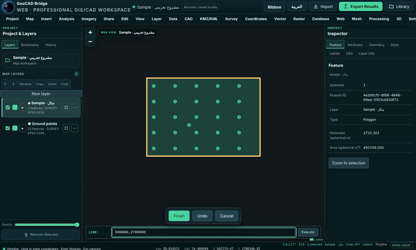
E,N– absolute point, for example562600,2703050.@ΔE,ΔN– relative to the last point, for example@25,0.@distance<angle– polar, for example@30<90(30 m at 90°).
Example – draw a 25 m × 15 m building outline by coordinates (project in a UTM CRS):
- Type
POLand press Enter. - Type
562600,2703050Enter, then@25,0Enter,@0,15Enter,@-25,0Enter. - Press Enter on the empty line to finish. Select it: the Inspector shows a perimeter of about 80 m and an area of about 375 m² (the Inspector values are spherical, so they differ very slightly from the grid values).
Part 3 (continued) · Ribbon reference, tab by tab
Every tab is listed in the order it appears on the ribbon. For each group, every command is described with what it opens or does. Commands marked (not available in this version) are shown greyed out.
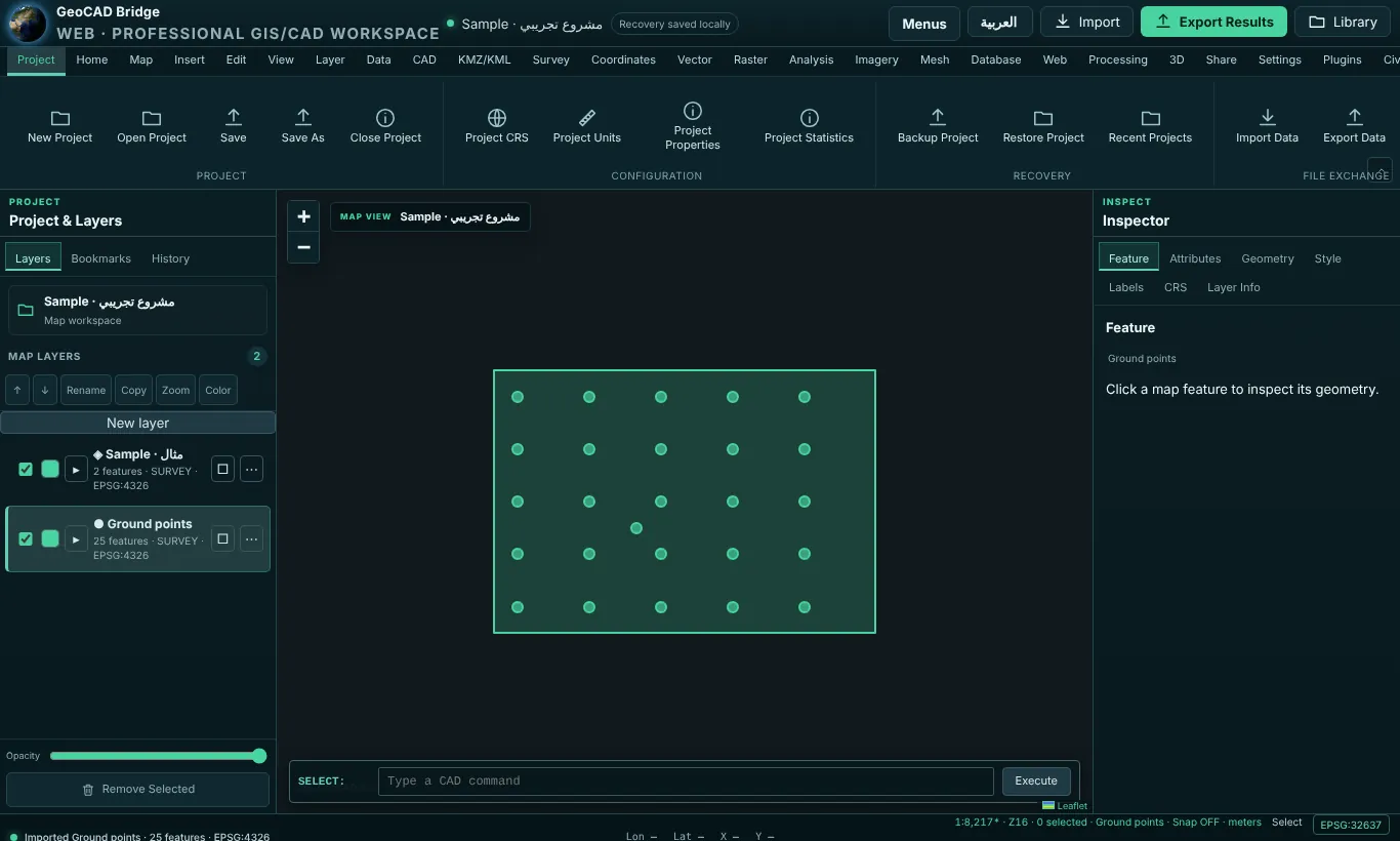
Project tab
| Group | Command | What it does |
|---|---|---|
| Project | New Project | Shows Work without an account (Start Project, How to Save a Project, Got it), then creates a new project. Shortcut Ctrl+N. |
| Open Project | Choose a .gcbproject file. Ctrl+O. |
|
| Save | Downloads the complete project file. Ctrl+S. | |
| Save As | Asks for a Project name and downloads a copy. Ctrl+Shift+S. | |
| Close Project | Returns to the Project Manager. | |
| Configuration | Project CRS | Opens the coordinate library. |
| Project Units | Report units: meters or feet. | |
| Project Properties | Name, Location, Description, Report units. | |
| Project Statistics | Table: Layer, Features, CRS. | |
| Recovery | Recover Autosave | Restores the temporary copy this browser keeps of the last project. |
| Recent Projects | Shows the Project Manager with the recent projects list. | |
| File exchange | Import Data | Import dialog. |
| Export Data | Export dialog. | |
| Print Map | Prints the map view with the browser’s print dialog. | |
| Project output | Report | Survey report table: Name, Geometry, Length (m), Area (m²), Layer, with Download CSV. |
Home tab
| Group | Command | What it does |
|---|---|---|
| Project | New Project, Open Project from File, Save Project to File | As above. |
| Data exchange | Import, Export Results | Import and export dialogs. |
| Navigate | Select | Selection tool. |
| Extents | Zoom to all data. | |
| Go To Coordinates | Choose a Coordinate system, type X / Easting / Longitude and Y / Northing / Latitude, Apply: the map centres on that point and marks it. |
Map tab
| Group | Command | What it does |
|---|---|---|
| Navigate | Explore, Pan Map | Pan and zoom the map (drag, mouse wheel). |
| Extents | Zoom to all data. | |
| Go To XY | Same as Go To Coordinates. | |
| Selection | Select | Selection tool. |
| Identify Features | Shows the details of exactly one selected feature in the Inspector. | |
| Clear Selection | Deselects everything. | |
| Layer | Add Data | Import dialog. |
| Layer Statistics | Geometry statistics of the active layer: Type, Features. | |
| Layer Color | Pick a colour for the active layer. | |
| Basemap | Bookmarks | Lists saved views (No bookmarks saved when empty). |
| Add Bookmark | Saves the current view under a Name. |
The basemap (streets, satellite, none) is chosen with the basemap control on the map. If a basemap provider cannot be reached, the Workspace switches to another one and tells you.
Insert tab
| Group | Command | What it does |
|---|---|---|
| Project items | New Project, Open Project | As above. |
| Project Manager | Shows the Project Manager. | |
| Add data | Data Source Manager, Import GIS / CAD | Import dialog. |
| Import Excel | Choose an Excel workbook. | |
| Coordinate List | Table of every point: ID / Name, X, Y, Z, Layer in the project CRS, Download CSV. | |
| Create features | Point, Polyline, Polygon, Rectangle, Circle | Drawing tools. |
| Layouts & reports | New Print Layout | Print the map. |
| New Report | Survey report table. | |
| Layout Manager | (not available in this version) |
Edit tab
| Group | Command | What it does |
|---|---|---|
| Selection | Select | Select a feature · Shift-click to select several. |
| Edit Attributes | Edit the fields of exactly one selected feature. | |
| Delete Feature | Delete the selection. | |
| Geometry editing | Edit Vertices | Move the vertices of one selected feature. |
| History | Undo, Redo | Ctrl+Z, Ctrl+Y. |
| Sketch control | Finish, Cancel | Enter, Esc. |
| Layers | Delete Layer | Deletes the active layer (after confirmation). |
| Rename Layer | New Layer name. | |
| Duplicate Layer | Copies the active layer. | |
| Clipboard | Cut Features, Copy Features | Put the selection on the clipboard. |
| Paste Features | Paste into the active layer. | |
| Feature editing | Add Polygon Feature | Polygon tool. |
View tab
| Group | Command | What it does |
|---|---|---|
| Map | Extents | Zoom to all data. |
| Full Screen | Browser full screen (Esc to leave). | |
| Panels | Explorer, Properties | Show or hide the Layers panel and the Inspector. Layer Visibility and Panels are not available in this version. |
| Map aids | North Arrow, Scale Bar | Show or hide them on the map. |
| Locations | Add Bookmark, Bookmarks | Save and list views. |
| Map navigation | 3D Map Views, Refresh | View and redraw commands. New Map View is not available in this version. |
Layer tab
| Group | Command | What it does |
|---|---|---|
| Data source | Data Source Manager, Add Layer | Import dialog. |
| Bridge Panel | The Bridge panel (see Survey panels). | |
| Create Layer | An empty layer for drawing or pasting features – type a Layer name. | |
| Georeferencer | (not available in this version) | |
| Attributes | Open Attribute Table | The attribute table of the active layer. |
| Filter | Filter features: Layer, Attribute, Condition (=, ≠, >, ≥, <, ≤, contains, starts with) and Value. Matching features are copied to a new layer; numbers are compared as numbers, text without regard to case. | |
| Layer Properties | Name, location, description, report units. | |
| Editing | Toggle Editing | Locks or unlocks the active layer. |
| Save Layer Edits | Downloads the complete project file. | |
| Remove Layer | Deletes the active layer. | |
| CRS & labeling | Set Layer CRS, Set Project CRS from Layer | Coordinate library (see Coordinate systems). |
| Labeling | Label settings for the active layer. |
Example – filter. Layer Ground points, Attribute code, Condition =, Value GS → a new layer with all 25 points coded GS.
Data tab
| Group | Command | What it does |
|---|---|---|
| Exchange | Import Dataset, Export Dataset | Import and export dialogs. |
| Import Excel | Choose a workbook. | |
| Export Excel | Downloads the active data as .xlsx at once. |
|
| Attributes | Attribute Table | Table with a Select column, ID and every field; Zoom selected, Edit selected, Export checked CSV, Previous / Next pages, search and sort. |
| Edit Attributes | Edit one selected feature. | |
| Layer Statistics | Geometry types and counts. | |
| Layer | Remove Layer | Deletes the active layer. |
| Project QA/QC | Project Templates | Create Project from Template: Building Survey or Utility Inventory. |
| Run QA/QC | QA/QC settings, then the project check (see below). | |
| Fields & validation | Field Calculator | Safe field tools (see below). |
| Validate Geometry | Table Feature, Finding listing invalid geometry. | |
| Spot Level | Spot Level | A labelled spot-level point at the map centre: Point number / label, Reduced level / elevation (m), Description. |
| Spot Point | A point at typed coordinates in the project CRS: label, Easting, Northing, Elevation / Z (optional), description. | |
| Level Label | Turns on elevation labels for the active layer. | |
| Elevation Difference | From and To elevation → the difference. | |
| Slope / Grade % | Elevation difference and Horizontal distance → grade in % and as a ratio. | |
| Interpolate Level | Start level, End level, Station from start, Total length → the level at that station. | |
| Level Report | Table: Feature, Label, Elevation, Description, Download CSV. |
Field Calculator (Field tools / safe calculator) applies to every feature of the active layer. Choose the Operation: Set constant, Copy field, Add numeric constant, Classify threshold, Concatenate, Area (m²), Length (m), Delete field, Rename field; then the Target field name, the Source field and the Value / suffix / numeric increment / threshold. Numeric operations validate all rows before anything is written. No JavaScript expressions are evaluated.
Example: Operation Add numeric constant, Target level_new, Source Z, Value 0.150 → every point gets its level raised by 15 cm in a new field.
Spot level examples.
- Elevation Difference: from
615.200to618.950→ +3.750 m. - Slope / Grade: elevation difference
1.5, horizontal distance60→ 2.5 % (1 : 40). - Interpolate Level: start
100.000, end102.000, station25, length100→ 100.500 m.
QA/QC. The settings dialog asks for the Duplicate-point tolerance in metres (0 disables) and an optional project extent (west, south, east, north in WGS 84). Run project check lists duplicates, empty or invalid geometry, missing CRS and features outside the extent. The check never changes features. The summary is stored in the project file.
CAD tab
| Group | Command | Shortcut | What it does |
|---|---|---|---|
| CAD exchange | Import DXF | Choose a DXF file directly. | |
| Export DXF | Export dialog (Choose scope and CRS, then select DXF). | ||
| Draw | Point | PO | Click or type E,N. |
| Polyline | PL | Click or type vertices; Enter finishes. | |
| Polygon | POL | Closed shape. | |
| Rectangle | REC | Two opposite corners. | |
| Circle | C | Centre and radius point. | |
| 3-Point Arc | A | Start, middle and end point. | |
| Ellipse | EL | Centre, then the axes. | |
| Freehand | FH | Free sketch. | |
| Construction Line | XL | Infinite helper line through two points. | |
| Modify | Transform | M / CO / RO / SC / MI | Move, copy, rotate, scale or mirror the selection. |
| Move | Move features: shift the selection by ΔE / ΔN on the project grid. | ||
| Rotate | Rotate features: rotate the selection by an angle (DMS accepted) about a base point. | ||
| Offset | Parallel copy of each selected line at a Distance (positive = right of the line direction), with mitred corners. | ||
| Edit Vertices | V | ||
| Delete | Delete / E | ||
| Undo, Redo | Ctrl+Z / U, Ctrl+Y | ||
| Drafting | Snap | F3 | Snap ON · F3. |
| Ortho | F8 | Ortho ON · F8. | |
| Finish, Cancel | Enter, Esc | ||
| Measure | Distance | DI | Click points; the running length is shown. |
| Area | AA | Click a polygon; area and perimeter are shown. |
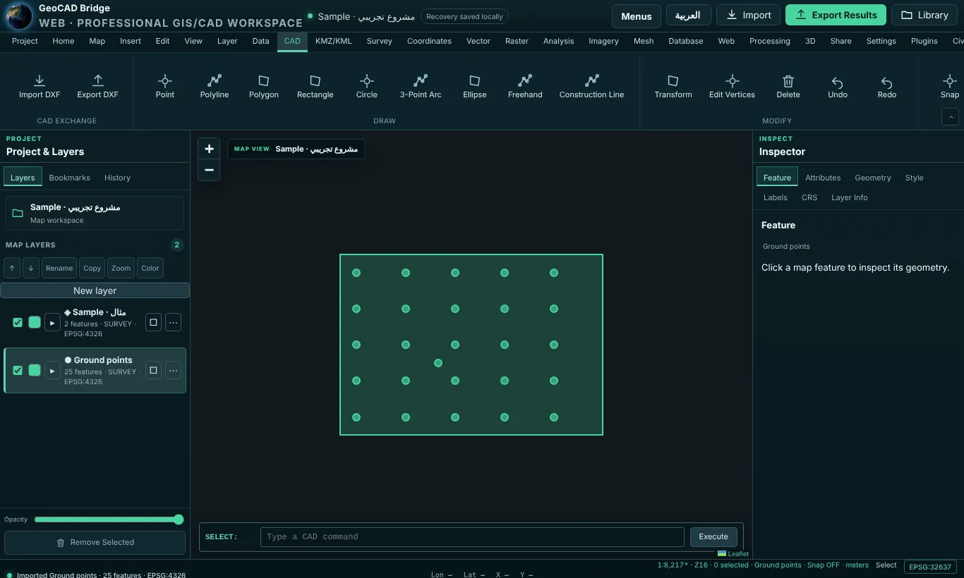
KMZ/KML tab
| Group | Command | What it does |
|---|---|---|
| Import | Import KML, Import KMZ, Import Google Earth File | Import dialog. |
| Export | Export KML, Export KMZ, Export Selected Layers | Export dialog (choose KML or KMZ). |
| Conversion | CSV to KML, DXF to KML, GEOJSON to KML | Import the source file, then export it as KML/KMZ. |
| KML to CSV | Export dialog: choose CSV. | |
| KML editing | Validate KML | Checks that features can be written to KML, for example 25 features are valid for KML (WGS 84 longitude, latitude). |
| Preview in Map | Zooms to the data. | |
| Style Placemarks | (not available in this version) |
Example – DXF to Google Earth. DXF to KML → choose the DXF → confirm its CRS (for example EPSG:32637) → Export KML → Scope Entire project → Google Earth · KMZ. Open the KMZ in Google Earth; the lines appear in the right place because the DXF grid coordinates were transformed to WGS 84.
Survey tab
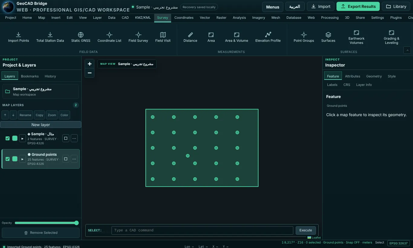
| Group | Command | What it does |
|---|---|---|
| Field data | Import Points | Import dialog (CSV / Excel / LandXML points). |
| Field Book (.fbk) | Opens a survey field book (see Opening a field book). | |
| Total Station Data | Survey Data Processor (see Survey panels). | |
| Static GNSS | Static GNSS Processing (see Survey panels). | |
| Coordinate List | All points in the project CRS, Download CSV. | |
| Field Visit | Opens the /field-visit-survey/ page (the browser asks before leaving the Workspace – save first). |
|
| Measurements | Distance, Area | Measuring tools. |
| Area & Volume | Area & Volume panel. | |
| Elevation Profile | Profile along a selected line (needs a layer with a line). | |
| Surfaces | Point Groups, Surfaces, Earthwork Volumes | The Surfaces & quantities panel on its three tabs. |
| Grading & Leveling | Grading panel. | |
| Traverse & COGO | Traverse Adjustment | Quick forward traverse: Start Easting, Start Northing, and one leg per line as grid bearing degrees, distance meters. Creates the traverse line and stations. No adjustment or ground scale correction. |
| Grid Bearings | For selected lines/polygons: table Feature, Segment, Grid bearing (°), Distance (m), Download CSV. | |
| Grid Stakeout | From a Station Easting / Northing to selected points: grid bearing and horizontal distance to each point. | |
| COGO Compute | Opens the Survey Calculators page in a new tab. | |
| Deliverables | Bridge Panel | Bridge panel. |
| PDF Report | Downloads the survey PDF report of the project. | |
| Report Branding | Company / office, Engineer, Licence / syndicate no., Phone / e-mail and logo images (PNG or JPEG up to 400 KB) shown on every PDF report. | |
| Survey Report | Table: Name, Geometry, Length (m), Area (m²), Layer. | |
| Export Points | Export dialog (choose PNEZD for Civil 3D / TBC). | |
| QA/QC Check | QA/QC settings and check. |
Example – Traverse Adjustment (forward traverse). Start E 500000, N 2700000, legs:
45, 100
135, 100
225, 100
315, 100
The result is a square of 100 m sides that closes on the start point.
Coordinates tab
| Group | Command | What it does |
|---|---|---|
| CRS library | Coordinate Systems Library | Opens the File Library. |
| Set Project CRS | Coordinate library. | |
| Validate CRS | Confirms the project CRS. | |
| Transform | Transform Coordinates, Batch Coordinate Converter | Coordinate transformation: Source CRS, Target CRS, X / Easting / Longitude, Y / Northing / Latitude → Apply shows the converted pair. For files use the site’s Batch Converter page. |
| Go To Coordinates | Centre the map on a coordinate. | |
| Formats | Decimal to DMS | Decimal degrees and Seconds decimals → DMS. |
| DMS to Decimal | Accepts 24°42'48.78"N, 24 42 48.78 or -46:40:… → decimal degrees. |
|
| UTM Zone Finder | Go-to dialog: enter a longitude/latitude to see its UTM zone in the Inspector. | |
| Quality | Axis Order Check | Layer extents per source CRS with a result. |
| Projection Report | Survey report table. | |
| CRS Audit | Checks the CRS of every layer against the project CRS. |
Examples. Decimal to DMS: 24.713611 with 2 decimals → 24°42′49.00″. Transform: Source EPSG:4326, Target EPSG:32638, X 46.5, Y 24.0 → E 652578.355, N 2655039.017.
Vector tab
| Group | Command | What it does |
|---|---|---|
| KML tools | KML Import, KML Export | Import / export dialogs. |
| KML/KMZ Converter | Opens the KML converter. | |
| Analysis tools | Buffer | Radius (meters); spherical buffer, the result is a new WGS 84 layer. |
| Clip | Clips the active layer by an Overlay polygon layer; result in a new layer. | |
| Points in Polygons | Table: Polygon, Layer, Point count (boundary included). | |
| Geometry tools | Check Geometry | For example No problems found in 25 features. |
| Fix Geometry | Repairs a copy of the layer (nothing needed fixing; a copy was added). | |
| Geometry Properties | Geometry statistics. | |
| Data management | Coordinate List, Export Layer | As above. |
| Reproject Layer | Copy of a layer in another coordinate system (see Reproject Layer). |
Raster tab
| Group | Command | What it does |
|---|---|---|
| Raster tools | Raster Calculator, Align Rasters, Raster Properties | (not available in this version) |
| Projections | Warp Reproject | Same as Reproject Layer. |
| Assign Projection | Coordinate library. | |
| Extract Projection | Table Projection · EPSG:…: Item, Value. | |
| Extraction & conversion | Clip Raster, Contour, Raster to Vector | (not available in this version) |
Analysis tab
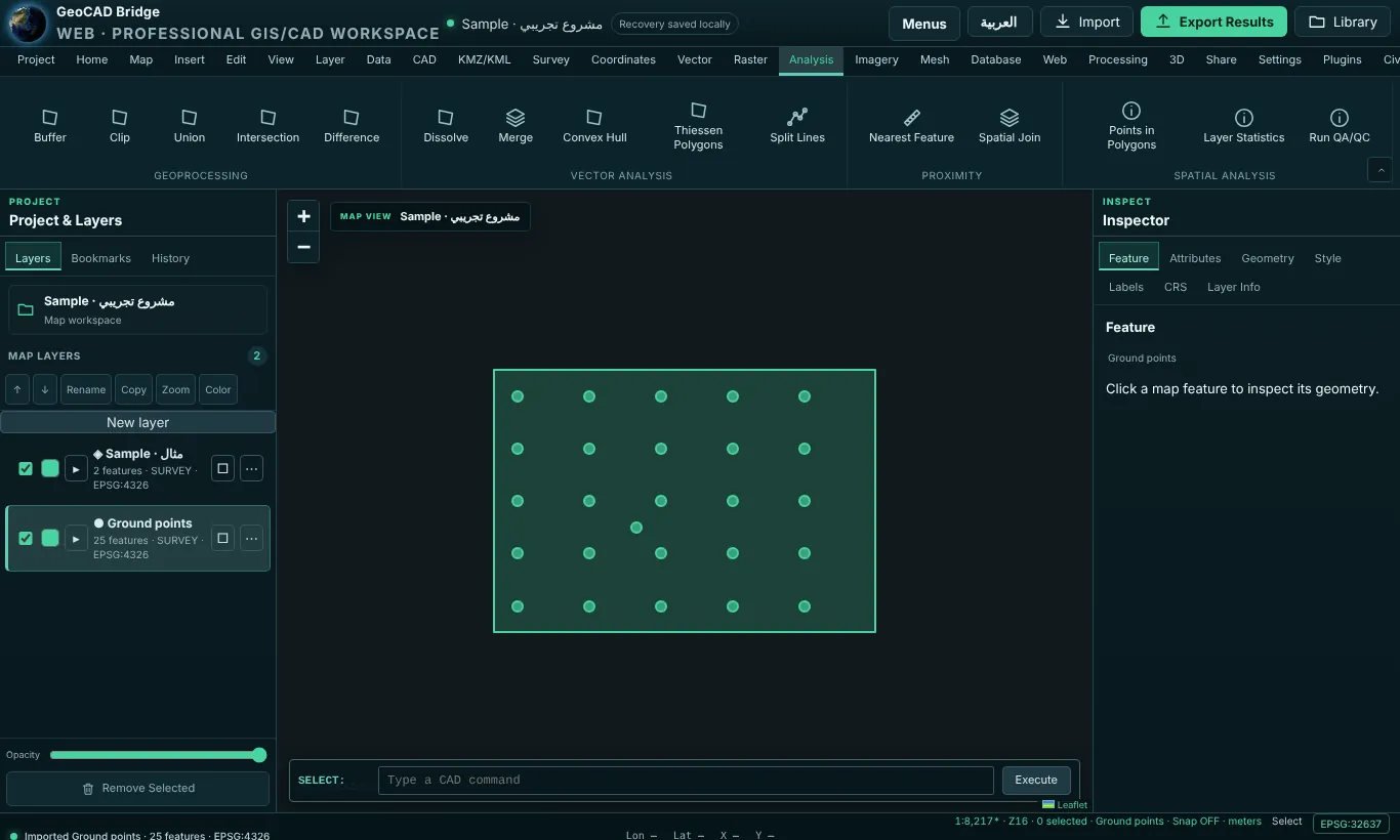
| Group | Command | What it does |
|---|---|---|
| Geoprocessing | Buffer | As in Vector. |
| Clip, Intersection, Difference | Choose the Overlay polygon layer; source geometries stay unchanged and the result goes to a new layer. | |
| Union | Union of polygon layers (Polygon layers are required). | |
| Vector analysis | Dissolve | Polygon layer and Dissolve by attribute (blank merges all); shared boundaries are removed. |
| Merge | First layer + Second layer → a new layer; a source_layer field records where each feature came from. |
|
| Convex Hull | The smallest convex polygon around the active layer. | |
| Thiessen Polygons | Voronoi cells around the points of a Point layer, on the project grid, clipped to the extent plus 10 %; each cell keeps the point attributes and gets its grid area. | |
| Split Lines | Splits lines at their vertices (needs a line layer). | |
| Proximity | Nearest Feature | From the centroid of each feature in one layer to the nearest feature of another; creates connector lines with the distance (grid distance when the project CRS is projected). |
| Spatial Join | Each point gets the attributes (join_*) of the polygon containing it, plus join_count. |
|
| Spatial analysis | Points in Polygons, Layer Statistics | Tables. |
| Run QA/QC | QA/QC check. | |
| Survey calculations | Total Station Data, Static GNSS, Area & Volume, Surfaces, Grading, Traverse, Traverse Correction, Grid Bearings, Grid Stakeout, Survey Report | The same tools as in the Survey tab. |
| Coordinates | Transform Coordinates, Go To Coordinates, Validate CRS | As in the Coordinates tab. |
Example – Thiessen polygons. With the 25-point Ground points layer, Thiessen Polygons → Point layer Ground points → Apply: a new layer of 25 cells, each with the point’s name, code and its grid area in m².
Imagery tab
| Group | Command | What it does |
|---|---|---|
| Raster data | Add Imagery | Import dialog. |
| Image Properties | Properties of a selected imagery layer. | |
| Georeference, Align Rasters | (not available in this version) | |
| Display | Swipe, Transparency, Enhance | (not available in this version) – use the layer Opacity slider for transparency. |
| Analysis | Raster Calculator, Classification, NDVI | (not available in this version) |
Mesh tab
| Group | Command | What it does |
|---|---|---|
| Mesh | Add Mesh Layer | Import dialog. Mesh Calculator and Mesh Properties are not available in this version. |
| Terrain | TIN Surface | Point layer with elevations and Elevation attribute (or Z coordinate) → a Delaunay TIN on the project grid; each triangle stores its corner elevations, grid area, slope and aspect. |
| Contours | Same inputs plus Interval (m) and Base level (m); contours are interpolated linearly across the TIN and every fifth one is an index contour. | |
| Surface Volume | Same inputs plus Reference level (m) → cut (surface above the level) and fill (below), exact for the TIN. Values are on the grid: multiply areas by the grid scale factor squared for ground values. | |
| Elevation Profile | Profile along a line. |
Example – contours. TIN Surface on Ground points using Z, then Contours with interval 1 and base 615 → contour lines at 615, 616, 617 … m, with every fifth line drawn heavier as an index contour.
Database tab
| Group | Command | What it does |
|---|---|---|
| Database | DB Manager, Query History, SQL Window | (not available in this version) |
| Connections | Add Connection | (not available in this version) |
| Import Table, Export Table | Import and export dialogs. |
Web tab
| Group | Command | What it does |
|---|---|---|
| Web layers | Add WMS/WMTS, Add XYZ Tiles, Add REST Map Service | (not available in this version) |
| Online data | EPSG Search | Opens the File Library / EPSG resources. |
| Coordinate Systems | Coordinate systems reference. | |
| Basemap Gallery | Basemap choice. |
Processing tab
| Group | Command | What it does |
|---|---|---|
| Toolbox | Processing Toolbox, Recently Used, Model Builder | (not available in this version) |
| Vector categories | Vector Analysis, Vector Overlay, Vector Geometry, Vector Selection | Jump to the matching Analysis / Vector tools. |
| Raster categories | Raster Analysis, Raster Creation, Raster Terrain | Jump to the Raster and Mesh tools. |
| Survey & CAD | Total Station Data, Static GNSS, Traverse, Coordinate Transform, CAD/GIS Conversion | Survey processors, transformation dialog and import dialog. |
3D tab
| Group | Command | What it does |
|---|---|---|
| 3D scene | Full Screen Scene | Full screen. New 3D View and Scene Properties are not available in this version. |
| Elevation | DEM / Terrain | Import dialog. |
| Elevation Profile | Profile along a line. | |
| Vertical Exaggeration | (not available in this version) | |
| 3D layers | Extrude Features, Point Cloud, 3D Tiles | (not available in this version) |
| Camera | Fly To Layer | Zooms to the active layer. Orbit is not available in this version. |
| Export 3D View | Export dialog (3D points keep Z in CSV, PNEZD, DXF and LandXML). |
Share tab
| Group | Command | What it does |
|---|---|---|
| Export | Bridge Panel | Bridge panel. |
| Export Map | Export dialog. | |
| Export Excel | Downloads .xlsx. |
|
| Print Map | Print. | |
| Packages | Save Project File, Save Copy, Project Properties | Project file commands. |
| Reports | PDF Report, Report Branding, Survey Report | As in the Survey tab. |
| Activity History | Table: Time, Action. | |
| Supported Formats | What the project file contains and every import/export format. |
Settings tab
| Group | Command | What it does |
|---|---|---|
| Preferences | Display Preferences | Interface density (comfortable / compact) and Status coordinates (Show / Hide). |
| Change language | English ⇄ Arabic interface. | |
| Report Units | Meters or feet. | |
| Keyboard Shortcuts | The shortcut list. | |
| Workspace | Toggle Ribbon | Collapses / expands the ribbon. |
| Reset Layout | Restores the default ribbon and panels. | |
| Editing | Snapping | Snapping On/Off, Target (Vertex, Endpoint, Midpoint, Segment), Screen tolerance (pixels). |
| Application | Custom Projections | Coordinate library. User Profiles and Style Manager are not available in this version. |
Plugins tab
| Group | Command | What it does |
|---|---|---|
| Plugins | KML/KMZ Converter | KML converter. Plugin Manager and Python Console are not available in this version. |
| Extensions | Install Tools, Manage Toolboxes, Developer API | (not available in this version) |
Help tab
| Group | Command | What it does |
|---|---|---|
| User Guide | Open User Guide | The in-app guide (in Arabic): each operation, the columns it needs and notes. |
| Reference | Import Templates | Column tables and the four CSV templates (survey-points.csv, traverse-coordinates.csv, traverse-observations.csv, geographic-points.csv). |
| Keyboard Shortcuts | Shortcut table. | |
| Support | Contact Us | Form: Name, Email, Topic, Message, Send. Your e-mail is used only to reply. |
| What’s New | Release notes and known limits (for example, traverse least squares and error ellipses are not yet available in the Workspace; transformations that need grid-shift files are flagged as not survey-grade). | |
| About GeoCAD Bridge | Version and description. |
Part 3 (continued) · Survey panels in depth
Survey Data Processor (Total Station Data)
Open: Survey › Field data › Total Station Data (also Analysis and Processing tabs).
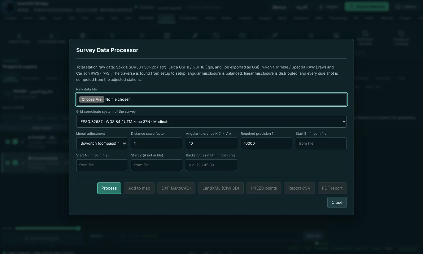
Reads total-station raw files: Sokkia SDR33 / SDR2x (.sdr), Leica GSI-8 / GSI-16 (.gsi, and .job exported as GSI), Nikon / Trimble / Spectra RAW (.raw) and Carlson RW5 (.rw5). The traverse is found from setup to setup; side shots are reduced from their setups.
Fields
- Raw data file – choose the file.
- Grid CRS – the system of the output coordinates (usually the project CRS).
- Linear adjustment – Bowditch or Transit.
- Distance scale factor – combined grid × elevation factor applied to distances (1 for none).
- Angular tolerance K – the allowed angular misclosure is K″ × √n (n = number of angles).
- Required precision 1: – for example 10000; the report says whether the traverse passes.
- Start E / N / Z and Backsight azimuth – needed only if the file does not contain them.
Buttons: Process → results (angular misclosure, linear misclosure, precision, adjusted stations and side shots) · Add to map · DXF · LandXML · PNEZD · Report CSV · PDF report.
Workflow. Choose the raw file → set the CRS and tolerances → Process → check the closure lines against your specification → Add to map → deliver DXF / LandXML / PNEZD for CAD and the PDF report for the client.
Static GNSS Processing
Open: Survey › Field data › Static GNSS.
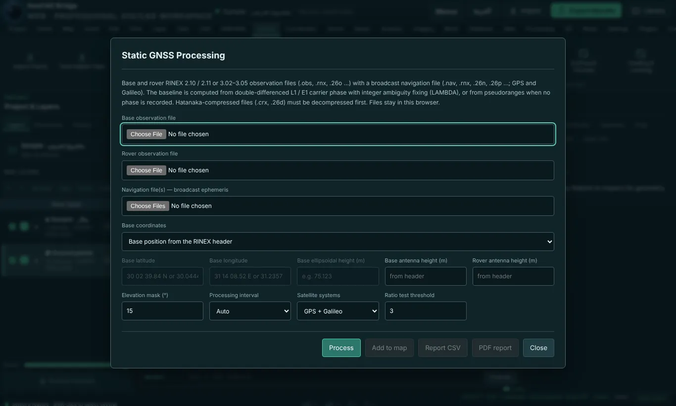
Inputs: base and rover RINEX 2.10 / 2.11 or 3.02–3.05 observation files (.obs, .rnx, .26o …) and a broadcast navigation file (.nav, .rnx, .26n, .26p …) for GPS and Galileo. The baseline is computed from double-differenced L1 / E1 carrier phase; ambiguities are fixed with LAMBDA when the ratio test passes.
Settings: base coordinates (from the RINEX header, or known WGS 84 latitude, longitude and ellipsoidal height), base and rover antenna heights, elevation mask (degrees), interval (Auto, All, 5–60 s), systems (GPS + Galileo, GPS only, Galileo only) and the ratio threshold for fixing.
Buttons: Process → the baseline (rover minus base) vector with its length and azimuth, the rover coordinates, the solution (Fixed, Float or Code only), the ratio test, RMS code (m) and RMS phase (mm), and the number of double-difference epochs · Add to map (GNSS points and the baseline line) · Report CSV · PDF report (static GNSS baseline report).
Limits. L1/E1 only; GLONASS and BeiDou are skipped; antenna phase-centre (ANTEX) models are not applied. Use it for short static baselines.
Area & Volume
Open: Survey › Measurements › Area & Volume.
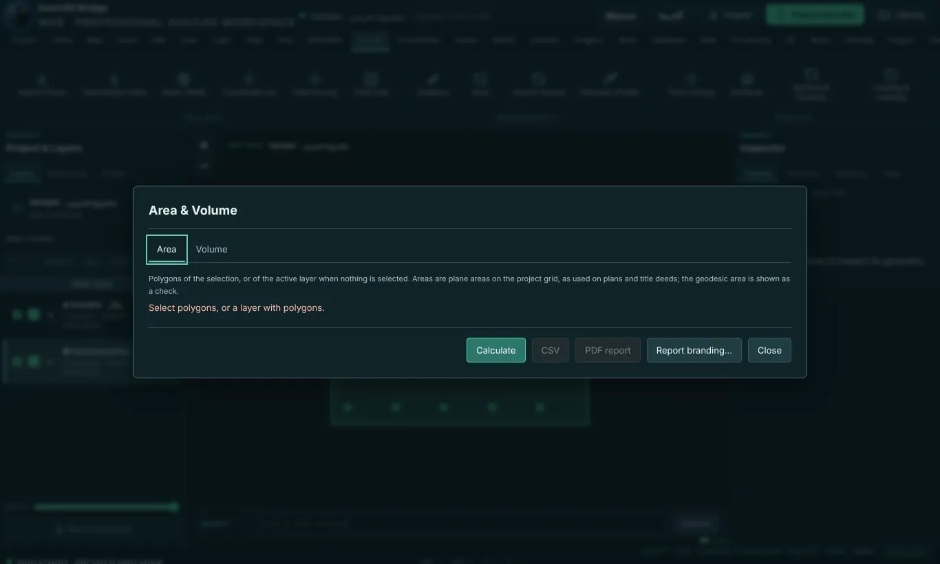
It works on the polygons of the selection, or of the active layer when nothing is selected. Areas are plane areas on the project grid, as used on plans and title deeds; the geodesic area is shown as a check.
- Area tab → Calculate: table of Area m², Hectares, Feddan · Qirat · Sahm (Egyptian units), Dunum and Perimeter for every polygon, with totals.
- Volume tab: choose the method – a prism (area × height), a TIN against a reference level, or cut/fill between two surfaces – then Calculate.
- CSV, PDF report, Report branding….
Example: a 100 m × 100 m plot = 10 000 m² = 1.0000 ha = 10.000 dunum = 2 feddan 9 qirat 3.2 sahm (1 feddan = 24 qirat = 576 sahm = 4 200.833 m²; 1 dunum = 1 000 m²).
Surfaces & quantities
Open: Survey › Surfaces › Point Groups / Surfaces / Earthwork Volumes.
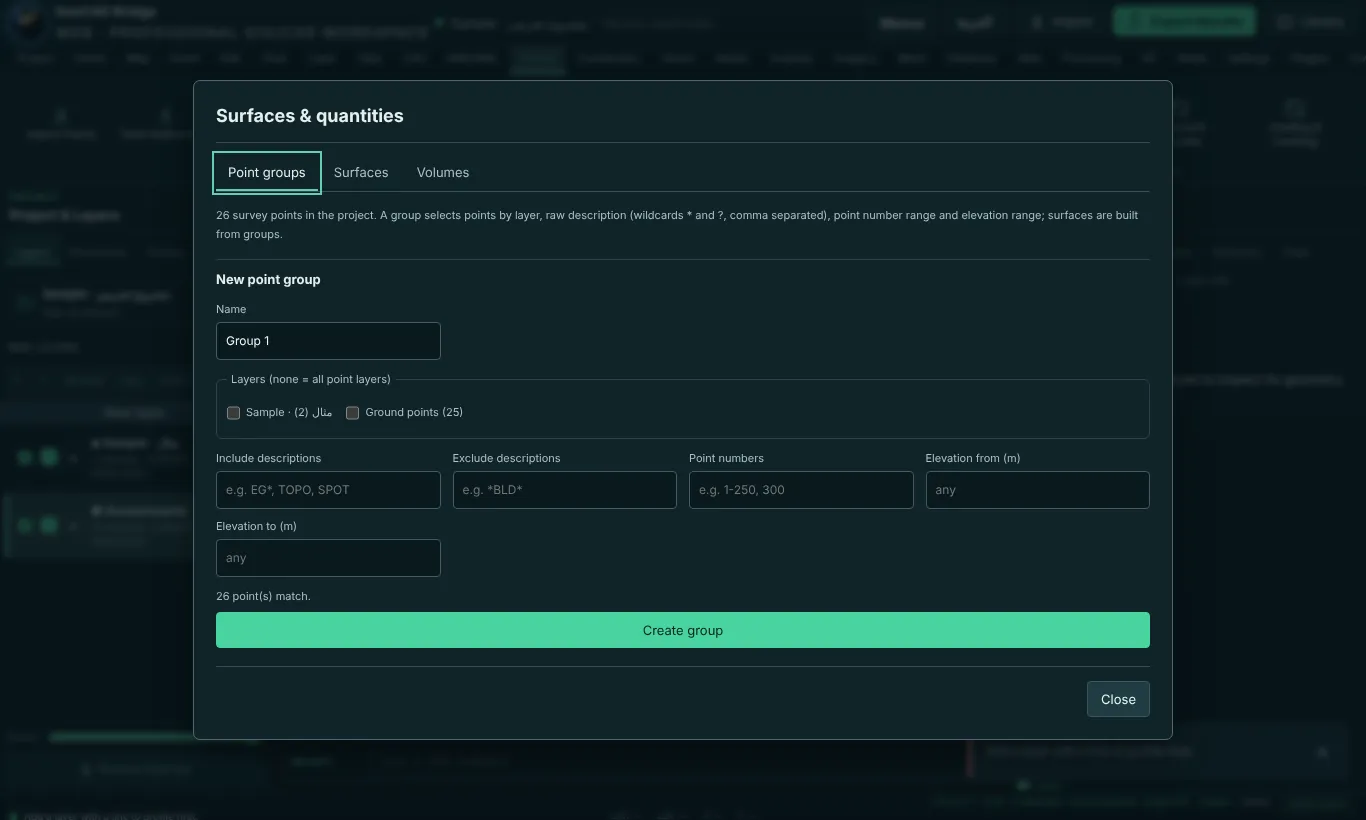
Point groups tab. A group selects points by layer, raw description (wildcards * and ?, comma separated, include or exclude), point number range and elevation range. Example: Name Ground, description GS*, elevation 600–700.
Surfaces tab. Create a TIN from point groups (all survey points when none is chosen) or a level plane. Options: outer boundary polygon, maximum triangle edge length, and breaklines (kept as triangle edges). Example: Name EG, Type TIN, group Ground, max edge 50 m.
Volumes tab. Needs two surfaces (for example existing ground EG and a design surface or a level plane). Methods: TIN to TIN (prismoidal, exact) or average end area from cross-sections along an alignment line with left/right widths and an interval. Results: cut, fill, net, a quantity table and contours. Create two surfaces first appears until both exist.
Grading & leveling
Open: Survey › Surfaces › Grading & Leveling.
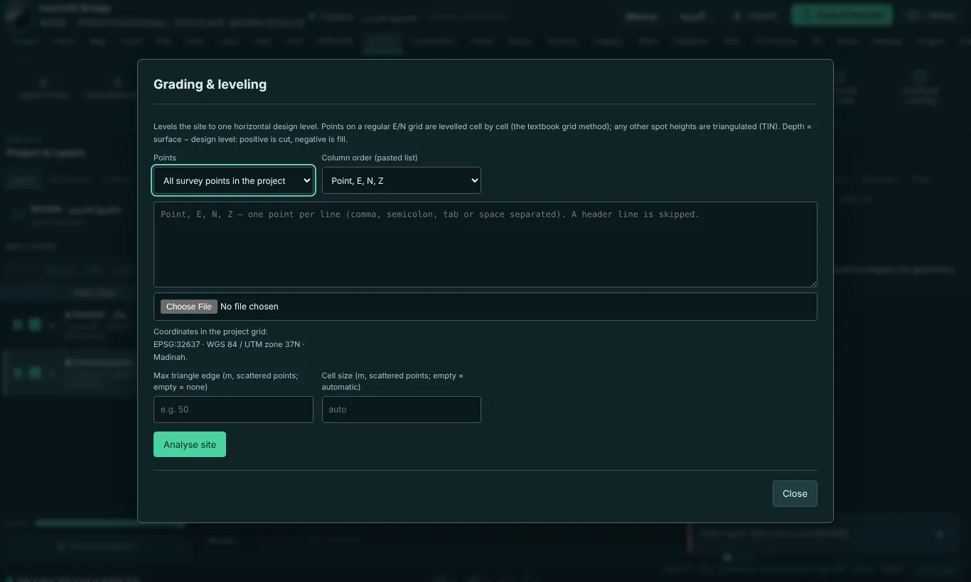
Levels the site to one horizontal design level. Points on a regular E/N grid are levelled cell by cell (the textbook grid method); scattered spot heights are triangulated (TIN). Depth = surface − design level: positive is cut, negative is fill.
- Points: All survey points in the project, or Paste or load a CSV / TXT list with a column order of
E,N,Z,Point,E,N,Z,Point,N,E,Z,N,E,ZorPoint,E,N,Z,Description. - For scattered points set the Max triangle edge and the Cell size (empty = automatic).
- Analyse site → the site area, minimum, maximum and mean level.
- Choose the design level: balanced (cut = fill), minimum earthwork, or a custom level.
- Compute → cut and fill volumes per cell and in total, the zero (daylight) line, and a coloured overlay on the map. Export the table or the PDF report.
Traverse Correction
Open: Analysis › Survey calculations › Traverse Correction.
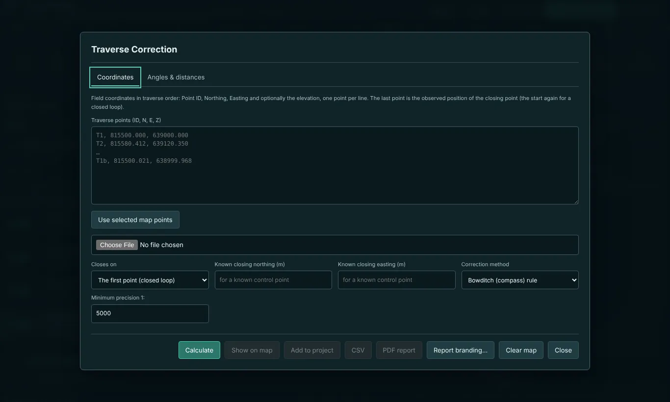
Two input modes:
- Coordinates: field coordinates in traverse order, one per line:
Point ID, Northing, Easting[, Elevation]. The last line is the observed position of the closing point (the start again for a closed loop). Coordinates carry no observed angles, so only the linear closure is checked. - Angles & distances: observed angles and distances, which gives both angular and linear closure.
Settings: Closes on The first point (closed loop) or A known control point (then type the known closing northing / easting), Correction method Bowditch (compass) rule, Transit rule or Least squares, and Minimum precision 1:.
Buttons: Use selected map points (fills the list from selected points), Calculate (step-by-step solution: misclosure ΔN, ΔE, linear misclosure, precision, corrections per leg, adjusted coordinates), Show on map, Add to project, CSV, PDF report, Report branding…, Clear map.
Least squares and error ellipses. In Angles & distances mode, choosing Least squares as the correction method runs a full network adjustment instead of distributing the misclosure leg by leg: enter the standard deviations you trust your angles and distances to (σ angle, default 5″, and σ distance, default 3 mm + 2 ppm), and the adjustment gives each point its most probable position together with its standard deviations in northing and easting, a 95 % error ellipse, and the network’s overall χ² (chi-square) goodness-of-fit test. Add to project adds the adjusted points with their σ values as attributes and an Error ellipses (95 %) polygon layer so the uncertainty is visible on the map; the PDF report lists every ellipse’s semi-axes and orientation. Least squares needs more redundancy than Bowditch (more observations than the minimum to fix the network) and is the method surveying authorities expect for boundary and control work.
Example (closed loop, coordinates mode):
A,2700000.000,500000.000
B,2700000.020,500100.010
C,2700100.030,500100.000
D,2700100.000,499999.980
A,2700000.040,500000.030
The closing point A is observed 0.040 m north and 0.030 m east of its start, a linear misclosure of 0.050 m over 400 m (precision 1:8 000). Bowditch distributes −0.040 m N and −0.030 m E in proportion to the cumulative leg length. With the default minimum precision of 1:5 000 the traverse passes. Adjusted coordinates (N, E): B 2700000.010, 500100.002 · C 2700100.010, 500099.985 · D 2700099.970, 499999.957, and A closes exactly on 2700000.000, 500000.000.
Bridge panel
Open: Survey › Deliverables › Bridge Panel, Layer › Data source › Bridge Panel, Share › Export › Bridge Panel, or a layer’s ⋯ › Bridge to AutoCAD / Civil 3D / QGIS / Trimble….
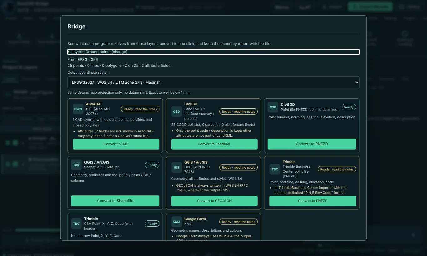
It shows, for each layer (name · feature count · CRS), what each target program will receive – Civil 3D, Trimble, QGIS / ArcGIS and Google Earth – and warns about anything that will be lost. Choose the Output coordinate system and click Convert to DXF, LandXML, PNEZD, Shapefile, GEOJSON, CSV or KMZ. An accuracy note travels with the file.
Geoid Heights
Open: Survey › Field data › Geoid Heights or Coordinates › Transform › Geoid Heights.
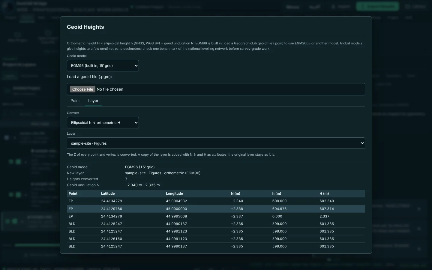
Converts between the GNSS ellipsoidal height h (WGS 84) and the orthometric height H (above mean sea level): H = h − N, where N is the geoid undulation of the chosen model at that point. Geoid model: EGM96 (15′ grid) and EGM2008 (5′ grid, generally more accurate) are built in; a GeographicLib geoid file (.pgm, up to 120 MB — for example a finer EGM2008 grid) can also be loaded from disk.
Two tabs:
- Point: enter a Latitude and Longitude (decimal degrees or D M S) and a Height, choose the direction (h → H or H → h), and Calculate shows the geoid undulation N and the converted height, with the formula used.
- Layer: choose a layer with 3D points and a direction; Calculate converts the Z of every point and vertex and adds a copy layer (the original is left untouched) with geoid_N, h_ellipsoid and H_orthometric attributes.
Both tabs can export the results as CSV. A global model gives heights to a few centimetres to decimetres (more in mountainous areas); check one benchmark of the national levelling network before survey-grade work.
Survey Plan
Open: Survey › Deliverables › Survey Plan.
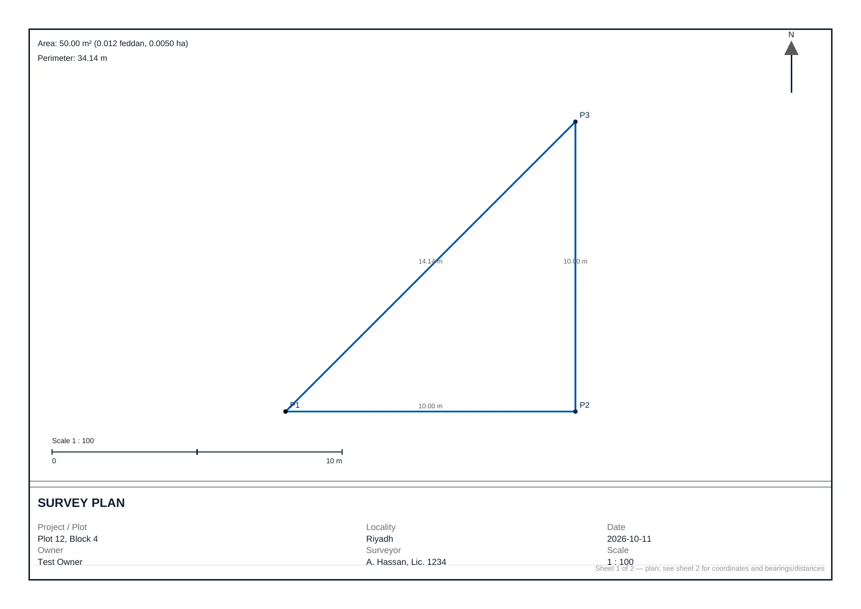
Builds an official-style parcel plan sheet automatically from a closed Boundary layer already in the project — a closed field-book figure, or an imported parcel polygon. Fill in the title block (Project / plot name, Owner, Locality, Surveyor, Date, Scale — leave blank for an automatic round scale that fits the sheet — and Paper size A4 or A3 landscape), then Build plan to compute every side’s bearing, azimuth and distance, the perimeter, and the area (m², hectares, feddan/qirat and acres).
PDF downloads a two-page sheet: page 1 is the plan itself (frame, title block, north arrow, the boundary drawn to scale with point labels and side distances, a scale bar, and the area/perimeter), page 2 lists every vertex’s coordinates and every side’s bearing, azimuth and distance. CSV exports the same coordinate and bearing/distance tables.
PDF report and Report branding
PDF Report (Survey › Deliverables, Share › Reports) downloads a PDF of the project’s survey results. Report Branding sets what appears on every PDF report: Company / office, Engineer, Licence / syndicate no., Phone / e-mail and up to two logo images (PNG or JPEG, ≤ 400 KB). Branding images stay in your browser only. Remove clears it.
Part 3 (continued) · Worked examples
Example 1 · From a CSV of survey points to Civil 3D and Google Earth
- Open the Workspace → New Project → name
Site A, CRS EPSG:32637. - Download
survey-points.csvfrom Help › Import Templates, fill it with your points (Point, Easting, Northing, Elevation, Description…) and save as CSV UTF-8. - Import → Survey · CSV Points → choose the file → confirm EPSG:32637.
- Check the points: Survey › Coordinate List; turn on labels in the Inspector’s Labels tab.
- Survey › Deliverables › Export Points → Scope Entire project, Output CRS EPSG:32637 → Civil 3D · TBC · PNEZD points. Import this file in Civil 3D with Import Points (PNEZD comma delimited).
- Export Results → Google Earth · KMZ for the client.
- Save Project to File to keep the work.
Example 2 · Convert a DXF from local grid to KSA-GRF17
- New project, CRS EPSG:9357 · KSA-GRF17 / UTM zone 37N.
- CAD › Import DXF, choose the drawing. Confirm the detected CRS; if the drawing is in WGS 84 / UTM 37N choose EPSG:32637.
- Look at the result on the basemap. Use Coordinates › Quality › Axis Order Check if it lands in the wrong place.
- Export Results → Output CRS EPSG:9357 → CAD · DXF.
Example 3 · Surface, contours and earthwork
- Import the levelling points (CSV with Z).
- Mesh › TIN Surface → point layer, Z → Apply.
- Mesh › Contours → interval
0.5, base0→ contour layer. - Survey › Surfaces › Grading & Leveling → Analyse site → Balanced → Compute → cut = fill volumes and the zero line.
- Share › Reports › PDF Report for the deliverable.
Example 4 · Close a traverse and deliver the report
- Survey the traverse; type the observed coordinates (or select the points on the map and use Use selected map points).
- Analysis › Survey calculations › Traverse Correction → Closes on: the first point, Bowditch, minimum precision
1:10000. - Calculate → read the misclosure and precision → Add to project.
- Report branding… with your office name and licence number → PDF report.
Example 5 · Process a total-station job
- Survey › Field data › Total Station Data → choose the
.sdr,.gsi,.rawor.rw5file. - Grid CRS = project CRS, Bowditch, scale factor (for example
0.9996), K =30, precision1:10000. - Process → check the closure → Add to map → DXF and PDF report.
Appendices
Appendix A · Template downloads
Appendix B · Keyboard shortcuts (Workspace)
| Keys | Command | Keys | Command |
|---|---|---|---|
| Ctrl + N | New project | Ctrl + Z | Undo |
| Ctrl + O | Open project | Ctrl + Y | Redo |
| Ctrl + S | Save project | Delete | Delete selected features |
| Ctrl + Shift + S | Save as | Esc | Cancel current tool |
| F | Zoom to selection | Enter | Finish drawing |
| F3 | Snap on/off | F8 | Ortho on/off |
| Shift + click | Multiple selection | F2 | Rename the selected layer |
Shortcuts are ignored while you are typing in an input field. The CAD command aliases are listed in The CAD command line.
Appendix C · Troubleshooting
| Problem | Cause and fix |
|---|---|
| Points appear in the sea or another country | The CRS is wrong or the axes are swapped. Run Coordinates › Quality › Axis Order Check, then Layer › Set Layer CRS with the right EPSG. For CSV, check that Easting and Northing are in the right columns. |
| A DWG file will not open | DWG is not read directly. Save it as DXF in AutoCAD (DXFOUT) and import the DXF. |
| Shapefile import fails | The ZIP must contain the .shp, .shx and .dbf with the same name. Add the .prj so the CRS is known. |
| Arabic text shows as ??? in CSV | Save the CSV as UTF-8. |
| I lost my project after closing the browser | The browser keeps only a temporary copy. Try Recover Autosave on the start screen. Always use Save Project to File. |
| Commands say Select features first | Select one or more features with Select (Shift-click for several), or make the right layer active. |
| A command is greyed out | It is not available in this version. |
| The basemap is blank | The tile provider is unreachable; the Workspace switches basemap automatically. Your data still draws. |
| Areas differ from another program | GeoCAD reports grid (plane) areas on the project CRS; spherical/geodesic areas are shown as a check. Make sure both programs use the same CRS. |
| The traverse misclosure is huge | Check the angle direction (clockwise / counter-clockwise), DMS typed as D.MMSS, and the order of the points. |